
- fMRI brain decoding
- Structural connectome
- Functional connectivity
- Dynamic inference
- Early exit
- Human Connectome Project
- Brain computer interfaces
- PyTorch
A volunteer lies in a scanner at one of the Human Connectome Project sites. A screen flashes a cue, and for the next ten seconds or so they tap fingers, listen to a story, or hold a picture of a face in working memory. Every 0.72 seconds the scanner returns a fresh volume of blood oxygen signal. Somewhere in that stream is the answer to a simple question that has kept decoding researchers busy for two decades. What is this person doing right now?
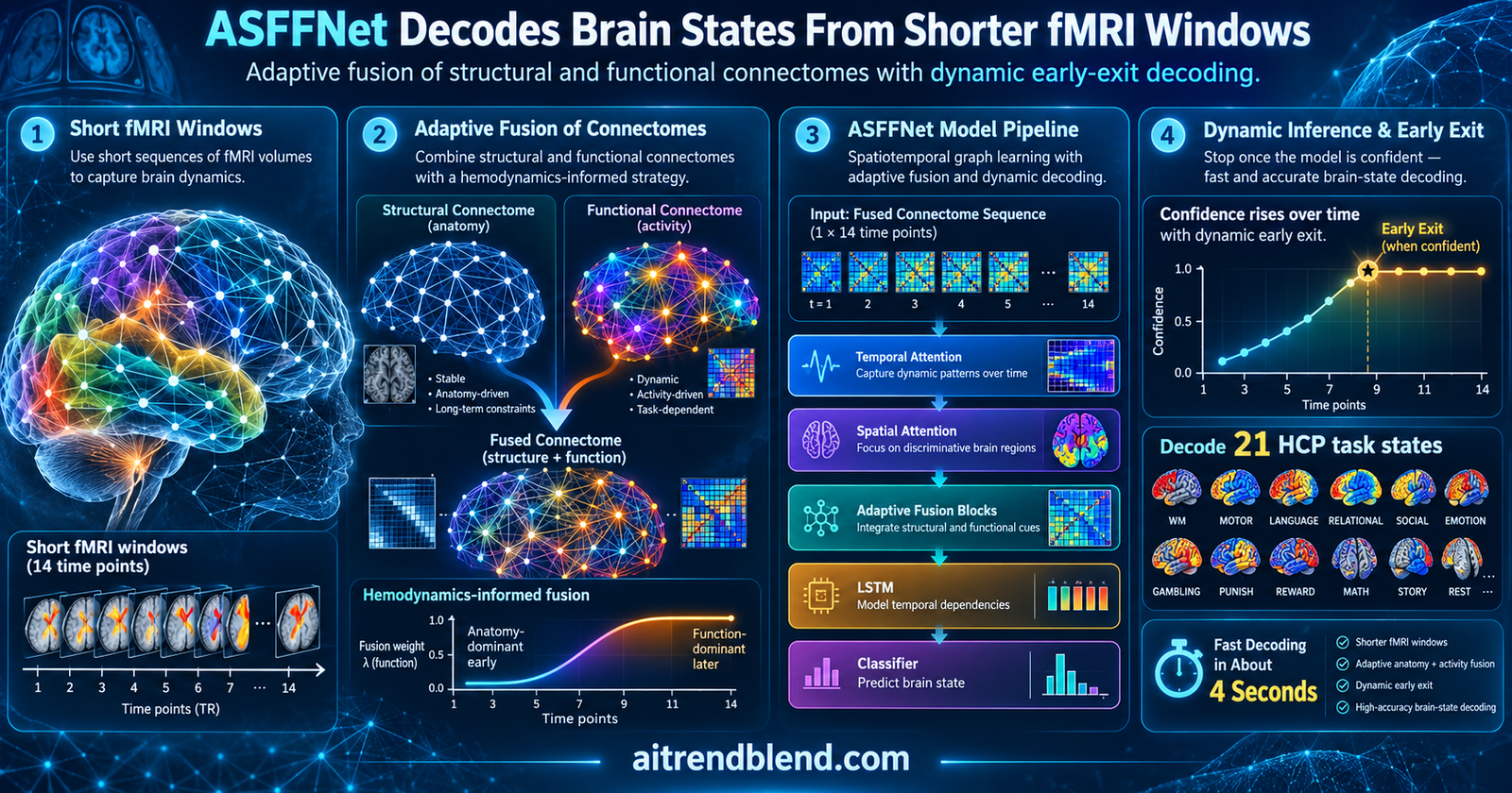
Most decoders answer only after a fixed number of volumes arrive, the same number for every task and every person. ASFFNet, from Chong Wang, Rong Li, Mingliang Xu, Huafu Chen and colleagues at the University of Electronic Science and Technology of China and Zhengzhou University, takes a different stance. It keeps reading until it is confident and then stops, and the brain graph it uses to share information between regions changes depending on how much of the scan it has seen.
Key points
- ASFFNet classifies 21 task conditions from Human Connectome Project fMRI using 360 cortical regions and a group structural connectome from diffusion MRI.
- A fixed sigmoid of input length hands control from the structural graph to a learned functional graph at about 5 seconds, the canonical hemodynamic delay.
- A confidence threshold lets each trial exit early. The model reports 85.79 percent accuracy with an average window of 4.05 seconds and 47.29 bits per minute.
- Gains over the strongest baseline, Graphormer, are real but moderate, around 2.3 points in static accuracy and 4.4 bits per minute in transfer rate.
- We recomputed the transfer rate from the reported accuracy and window and got 47.24 bits per minute, consistent with the paper. Our PyTorch reconstruction lands at 263 thousand parameters, close to the reported 0.27 million.
- The evaluation is offline on healthy young adults. Online preprocessing, hemodynamic lag and patient populations remain untested.
Please read. This article explains published neuroimaging research. It is not medical advice, diagnosis, or treatment, and ASFFNet is a research model rather than a clinical tool. Anyone with a health concern should consult a qualified professional.
Why a fixed window is the wrong assumption
The problem runs deeper than it first appears. Functional MRI does not measure neurons firing. It measures the slow swell of oxygenated blood that follows neural activity, and that swell takes several seconds to build. A decoder that sees only the first volume after a cue is looking at a brain that has barely begun to respond.
So the obvious move is to wait. But how long? Earlier work by Zhang, Tetrel, Thirion and Bellec found that the window you need depends on the task. In their graph convolution decoder, motor tasks reached a plateau within about 6 seconds, while working memory needed up to 14 seconds to get there. A single fixed window is therefore wrong in both directions at once. It wastes scan time on easy trials and cuts difficult trials short.
There is a second assumption hiding in the graph based decoders that ASFFNet builds on. Those models route information between brain regions along one connectivity matrix, usually derived from diffusion tractography or resting state correlations, and that matrix is identical for every trial. Neuroscience has known for years that it is not that simple. Mueller and colleagues showed sizeable individual variability in functional connectivity architecture, and task demands reshape which regions talk to which. A static graph treats the brain as a fixed circuit board.
ASFFNet attacks both assumptions together. It learns a functional graph per trial, mixes it with the anatomical graph according to how much signal is available, and lets each trial decide when it has seen enough. Whether those choices hold up is the interesting part.
What decoding looked like before ASFFNet
Early fMRI decoders worked on activation maps, which average many trials of a condition into one statistical image. That is fine for neuroscience but useless for anything that has to react to a single trial. Deep learning shifted the field toward end to end models that read raw single trial time series. Three dimensional convolutional networks classified four and seven cognitive states from fMRI volumes. Recurrent models, including the LSTM decoder of Li and Fan, showed that modelling temporal dynamics helps tell apart subtly different brain states.
The most recent jump came from graph neural networks. Zhang and colleagues, first in NeuroImage in 2021 and then with Farrugia and Bellec in Medical Image Analysis in 2022, treated cortical regions as nodes, fMRI responses as node features, and empirical connectomes as edges. Those models reported accuracy above 90 percent on the same 21 condition HCP benchmark that ASFFNet uses. The lesson the ASFFNet authors take from that line of work is that large scale cognitive decoding needs a connectome to integrate information across the cortex. The question they add is which connectome, and when.
If you follow our coverage of brain network models, you will recognise the shape of the debate. AdaPHBNA learned hierarchical brain networks from resting state fMRI for autism and depression diagnosis, and BRAINEXA modelled what a typical brain looks like so it could flag deviations without labels. ASFFNet sits on the other side of the fence. It reads task fMRI, and it cares about speed as much as accuracy, which pulls it toward the brain computer interface problems that EEG decoders like CD-CMAN usually own.
There is also a quieter influence from outside neuroscience. Dynamic neural networks, surveyed by Han, Huang, Song and colleagues in IEEE TPAMI, allocate computation per input instead of running every sample through the same fixed graph. Early exit classifiers in vision and text are the best known example. ASFFNet borrows that idea and applies it along the time axis of a scan, which turns out to be a natural fit for a signal that literally arrives one volume at a time.
How ASFFNet is built
The input is a matrix of 360 cortical regions by 14 time points. The regions come from the HCP multimodal parcellation, HCP_MMP1.0, which carves each hemisphere into 180 areas based on architecture, function, connectivity and topography. Fourteen time points at a repetition time of 0.72 seconds is a little over 10 seconds, chosen because it is the shortest trial length across all retained tasks. Alongside the fMRI comes a single structural connectivity matrix of 360 by 360, built from probabilistic diffusion tractography across 1065 HCP participants and normalised with a softmax across each row.
That row softmax is a small detail with a useful consequence. Each row now sums to one, so the structural matrix reads as the fraction of fibre tracts leaving region i that also pass through region j. The learned functional graph is also softmax normalised by row. Any weighted mix of the two therefore stays a proper averaging operator, which keeps feature magnitudes stable no matter how the mixing weight moves.
The network stacks three structure function fusion blocks, each made of a temporal attention module, a spatial attention module and an adaptive fusion module in series, followed by an LSTM and a linear classifier. The design follows the serial channel then spatial ordering of CBAM from Woo and colleagues, with the non local block of Wang, Girshick, Gupta and He supplying the functional graph.
Temporal attention decides which seconds matter
The first module squeezes out the spatial dimension. It takes the average and the maximum across all 360 regions at every time point, passes both 14 dimensional vectors through a shared two layer perceptron, adds them and applies a sigmoid. The result is one weight per time point, and the input is rescaled by those weights.
Here \(x \in \mathbb{R}^{N\times T}\), \(W_0\) and \(W_1\) are the perceptron weights shared by both pooled vectors, and \(\sigma\) is the sigmoid. Think of it as a learned prior over when the hemodynamic response is informative.
Spatial attention decides which regions matter
The second module does the mirror operation. It averages and maxes across time for each region, stacks the two resulting 360 element vectors as two channels, and runs a one dimensional convolution followed by a sigmoid to get one weight per region. A residual connection adds the original input back.
One design choice deserves a second look. A one dimensional convolution slides along the region index, so it assumes that regions with neighbouring indices are related. In a parcellation the index order is a labelling convention. Some neighbouring labels are cortical neighbours and many are not. The paper does not report the kernel size, and it does not discuss whether the ordering matters. A permutation test, shuffling region order and retraining, would settle it cheaply.
Adaptive fusion turns a dial between anatomy and activity
This is the heart of the model. The module first builds a trial specific functional graph using a non local attention block. Two 1 by 1 convolutions, \(\theta\) and \(\varphi\), project each region’s feature vector into an embedding space, and their dot products, passed through a softmax over regions, become a 360 by 360 affinity matrix. That matrix is a learned stand in for functional connectivity, computed from this trial alone.
Then comes the fusion. The functional graph and the structural graph are mixed with a weight \(\lambda\) that depends only on how many time points \(L\) the model has received. The mixed graph aggregates a third projection, \(g(x_S)\), across regions.
The number 7 is not arbitrary. Seven volumes at 0.72 seconds is 5.04 seconds, close to the textbook delay of the hemodynamic response function described by Friston and colleagues. Before that point the functional graph is estimated from almost no signal, so the model leans on anatomy. After it, the trial’s own connectivity takes over.
Here is where it gets interesting. Because \(\lambda\) is a plain logistic curve with unit slope, the handover is far sharper than the word adaptive suggests. We computed the schedule directly from Equation 9.
| Time points L | Seconds of fMRI | Functional weight λ | Structural weight 1 minus λ |
|---|---|---|---|
| 1 | 0.72 | 0.0025 | 0.9975 |
| 3 | 2.16 | 0.018 | 0.982 |
| 5 | 3.60 | 0.119 | 0.881 |
| 7 | 5.04 | 0.500 | 0.500 |
| 9 | 6.48 | 0.881 | 0.119 |
| 11 | 7.92 | 0.982 | 0.018 |
| 14 | 10.08 | 0.999 | 0.001 |
Table A. Fusion weights implied by Equation 9 of the paper, computed by the aitrendblend team. Almost the whole transition happens between roughly 3.6 and 6.5 seconds.
In practice ASFFNet runs two regimes with a short crossfade. Under about four volumes it is essentially a structural graph network. Past about ten it is essentially a non local attention network. Since the average dynamic exit lands at 4.05 seconds, which is between five and six volumes, many trials stop right inside the crossfade where both graphs carry real weight. That is probably not an accident, and it suggests the fusion matters most for exactly the trials that early exit makes common.
The LSTM reads only what actually arrived
After three fusion blocks, the 360 by 14 feature map is fed to an LSTM one time point at a time. Shorter inputs are padded with a learned token, but the authors pack the sequences with their true lengths so padded steps never update the recurrent state. The classifier reads the hidden state at the last valid step, not the last padded one. It sounds like housekeeping. It is also the difference between a model that genuinely handles variable length input and one that quietly learns to read padding.
The decoder does not ask how long a trial should be. It asks, after every new volume, whether it already knows the answer. aitrendblend analysis of ASFFNet, Information Fusion 2027
Confidence decides when to stop
Training runs in two phases. For the first 50 of 100 epochs the model only sees full 14 point inputs, so it learns solid representations before facing truncated ones. After that, each training step samples a random length between 1 and 14 and masks everything beyond it with the learned token.
At test time the model starts with one volume. If the top softmax probability clears a threshold for that length, the prediction is accepted. If not, the next volume is added and the check repeats, up to the full 14. The thresholds come from the training subjects of each fold using a simple quantile rule.
Here \(C_{sorted}\) is the list of training set confidences at length \(i\), sorted from highest to lowest, and \(N\) is the number of training samples. Read it slowly and the logic becomes clear. At length 1 the threshold sits at the top one fourteenth of training confidences, so only about 7 percent of training trials could exit there. At length 7, roughly half could. By length 14 the threshold falls to the lowest confidence, so everything exits. The schedule is a linear ramp in exit rate, imposed by hand.
That has two consequences worth naming. On training data, it caps the expected exit point near the middle of the window, about seven or eight volumes, and earlier for trials that are confident before their turn. The reported 4.05 second test average, between five and six volumes, fits that picture. And because training confidences are typically higher than test confidences on a model that has fit its training set, thresholds estimated this way tend to be strict on new subjects, which pushes exits later rather than earlier. The rule is sensible and leak free, since it never touches test subjects. It is not tuned to maximise transfer rate, which leaves room for a calibrated or validation tuned version to do better.
What the experiments show
The evaluation uses task fMRI from the HCP young adult release. Of seven task paradigms, gambling was dropped because its trials are too short, leaving motor, language, emotion, relational, social and working memory with 21 conditions in total. Some 1111 participants contributed at least one task. Splits are subject wise across ten folds, so no person appears in both training and test, and hyperparameters are chosen by nested cross validation on inner validation subjects only. That is a clean protocol and better than much of the decoding literature.
Five baselines were trained under the same procedure and split. GCN, ChebNet and Graphormer used fMRI and the diffusion connectome. A plain Transformer and MLP-Mixer used fMRI alone. Each had three layers, blocks or encoders to match ASFFNet’s three fusion blocks. The full results are published in the ASFFNet paper in Information Fusion, and the table below reproduces the headline numbers.
| Method | Params | Static acc % | Macro F1 % | Mean window s | Dynamic acc % | ITR bits/min |
|---|---|---|---|---|---|---|
| GCN | 0.14M | 71.87 ± 0.97 | 68.14 ± 1.14 | 3.97 | 75.23 | 38.02 ± 1.44 |
| ChebNet | 0.15M | 74.96 ± 1.10 | 71.54 ± 1.35 | 4.33 | 80.94 | 39.82 ± 1.88 |
| Transformer | 0.28M | 75.92 ± 0.83 | 72.91 ± 1.18 | 4.08 | 80.47 | 42.01 ± 1.49 |
| Graphormer | 0.28M | 78.01 ± 0.82 | 75.24 ± 0.99 | 4.30 | 84.03 | 42.87 ± 1.36 |
| MLP-Mixer | 1.61M | 71.10 ± 0.77 | 67.74 ± 0.94 | 3.83 | 73.22 | 37.61 ± 1.31 |
| ASFFNet | 0.27M | 80.31 ± 0.72 | 76.70 ± 0.82 | 4.05 | 85.79 | 47.29 ± 1.63 |
Table B. Static and dynamic decoding on 21 HCP conditions, from Table 2 of Wang et al. Static accuracy is averaged over all input lengths from one time point to the full window. ASFFNet beat every baseline at p below 0.001 by a Wilcoxon signed rank test.
The numbers tell a complicated story, in a good way. ASFFNet wins every column except mean window, where MLP-Mixer and GCN exit sooner but at a steep cost in accuracy. Its margin over Graphormer is 2.3 points in static accuracy and about 4.4 bits per minute in transfer rate, at almost the same parameter count. That is a solid and statistically supported gain. It is not an order of magnitude.
Readers comparing with the earlier GNN papers should be careful. The 80.31 percent static figure is an average over every window length, including single volume inputs where any decoder is close to guessing. It is not comparable with the above 90 percent figures that Zhang and colleagues reported at full length. In the paper’s own accuracy curve, ASFFNet with adaptive fusion climbs past 90 percent as the window approaches 10 seconds, which is the fairer comparison.
Dynamic inference earns its keep
The cleaner result is what early exit buys. At an average of 4.05 seconds of data, ASFFNet reaches 85.79 percent. The authors report that this is about 8.8 percent higher than static inference at the same window and comparable to static inference with 5.8 seconds of data. In other words, letting easy trials leave early and hard trials stay longer saves about 1.75 seconds of scan time per decision for the same accuracy.
We checked the transfer rate ourselves. Using the standard Wolpaw formula for 21 equally likely classes, an accuracy of 85.79 percent and a window of 4.05 seconds give 3.19 bits per decision out of a possible 4.39, which works out to 47.24 bits per minute. The paper reports 47.29, averaged over folds. The small gap is what you would expect from averaging per fold rates rather than computing one rate from averaged inputs.
The confidence signal also behaves the way an early exit system needs it to. Across every input length, correctly classified test trials carried higher confidence than misclassified ones, by 0.24 on average. That gap is what makes a confidence threshold meaningful at all. If wrong answers were as confident as right ones, stopping early would simply lock in mistakes.
Which fusion schedule works best
The authors also compared fusion strategies under dynamic inference. No fusion means the learned functional graph alone. Static fusion means a fixed equal weighting of the two graphs. Adaptive fusion uses Equation 9 with the delay parameter set to 0, 3, 7, 11 or 14 time points.
| Fusion setting | Mean window s | Dynamic acc % | ITR bits/min |
|---|---|---|---|
| Without fusion | 4.32 | 84.41 | 43.01 |
| Static fusion | 4.13 | 85.32 | 45.90 |
| Adaptive, delay 0 | 4.22 | 85.80 | 45.37 |
| Adaptive, delay 3 | 4.10 | 85.42 | 46.28 |
| Adaptive, delay 7 | 4.05 | 85.79 | 47.29 |
| Adaptive, delay 11 | 4.13 | 85.92 | 46.53 |
| Adaptive, delay 14 | 4.18 | 85.77 | 45.73 |
Table C. Fusion strategies under dynamic inference, from Table 4 of Wang et al. Delay 7 corresponds to 5.04 seconds, the canonical hemodynamic delay.
Adding the anatomical graph clearly helps. Going from no fusion to any fusion lifts transfer rate by roughly 2 to 4 bits per minute. The specific delay of 7 gives the best transfer rate and the shortest mean window, which supports the hemodynamic story. Delay 11 edges it on raw accuracy, though.
This is not a small distinction. The spread across delays from 3 to 14 is about one bit per minute, and this table reports no standard deviations, unlike Table B where fold to fold spread is around 1.4 to 1.9 bits per minute. So the evidence that 7 specifically is the right delay is suggestive rather than decisive. The evidence that fusing anatomy in at all is better than ignoring it is much stronger.
What each module contributes
| Removed component | Accuracy % | Macro precision % | Macro F1 % |
|---|---|---|---|
| Temporal attention | 79.71 ± 0.60 | 77.15 ± 0.76 | 76.02 ± 0.76 |
| Spatial attention | 79.68 ± 0.74 | 77.12 ± 0.93 | 75.96 ± 0.95 |
| Adaptive fusion | 77.90 ± 0.83 | 75.15 ± 0.95 | 74.11 ± 0.93 |
| LSTM | 78.79 ± 0.62 | 76.31 ± 0.78 | 74.92 ± 0.83 |
| Full model | 80.31 ± 0.72 | 77.77 ± 0.82 | 76.70 ± 0.82 |
Table D. Ablation from Table 3 of Wang et al. Every reduced model is significantly worse than the full model at p below 0.005.
The ranking is informative. Removing adaptive fusion costs 2.41 points, the largest drop, and removing the LSTM costs 1.52. The two attention modules each cost about 0.6. So the parts that carry the paper’s main idea, the graph mixing and the sequence model, are also the parts the network depends on most. The attention modules are polish.
ASFFNet’s strongest evidence is for two claims. Fusing a structural connectome into the decoder helps, and letting trials exit on confidence saves scan time at equal accuracy. The specific hemodynamic delay of 7 time points is supported, but the margin over nearby settings is within the noise one would expect from fold to fold variation.
On the practical side, the model runs in 2.50 milliseconds per forward pass on one RTX 5090 with 22.48 megabytes of peak memory. Against a repetition time of 720 milliseconds, compute is not the bottleneck. Hyperparameters barely matter either. Across temporal widths of 32 to 128, fusion channels of 8 to 32 and LSTM sizes of 128 or 256, accuracy stays essentially flat, with the best setting at 64, 32 and 128.
Does the model look at the right parts of the brain
Accuracy alone says little about whether a decoder found neuroscience or a shortcut. The authors probe this three ways, and the results are among the more convincing in recent decoding papers.
First, the temporal attention weights, averaged across test trials, look remarkably similar for all six tasks. They rise over the first few volumes, dip sharply around the fifth, then jump to saturation from the seventh time point onward, which is 5.04 seconds. The authors read the early part as resembling the canonical hemodynamic response and the flat tail as a consequence of block designs where the stimulus stays on. We would add that the shape is identical across tasks, which suggests the module has learned a generic timing prior rather than anything task specific.
Second, spatial saliency maps from the spatial attention module and from Grad-CAM++ were projected onto the cortical surface and correlated with the HCP’s official GLM activation maps, which serve as the reference since the GLM knows the true condition timing.
| Contrast | Spatial attention r | Grad-CAM++ r |
|---|---|---|
| Motor, average | 0.86 | 0.65 |
| Language, story versus math | 0.88 | 0.42 |
| Emotion, faces versus shapes | 0.85 | 0.38 |
| Social, theory of mind versus random | 0.80 | 0.39 |
| Relational, relational versus match | 0.74 | 0.30 |
| Working memory, 2 back versus 0 back | 0.48 | 0.17 |
Table E. Correlation between ASFFNet saliency maps and GLM activation maps, read from Figure 4 of Wang et al. All correlations were significant at p below 0.001.
The spatial attention maps track the GLM closely for motor, language, emotion and social tasks. Working memory is the weak spot at 0.48. Grad-CAM++ is consistently weaker, which is a useful reminder that different explanation methods applied to the same network can give different answers.
Third, network level saliency from the fusion module shows contralateral somatomotor hubs for hand movements, a left lateralised language hub, visual networks for the emotion task and frontoparietal dominance for working memory. Those are the patterns a neuroscientist would expect. To their credit, the authors frame all of this carefully. They cite the Jain and Wallace and Wiegreffe and Pinter exchange over whether attention counts as explanation, and they describe their results as qualitative indications of task sensitivity rather than proof of biological plausibility. That is the right level of claim.
The failure analysis lines up with the saliency results. In the confusion matrix, math trials in the language task are among the easiest at around 0.93 precision, while relational trials sit near 0.67 and the body 2 back condition near 0.63. Errors cluster inside a task paradigm rather than across paradigms. ASFFNet rarely mistakes a motor trial for a language trial. It does confuse 0 back and 2 back versions of the same stimulus category, which share most of their visual and attentional demands. The tasks where saliency matched the GLM least are the same ones where decoding was hardest, which is exactly the consistency you want to see.
What the paper does not settle
None of this comes for free, and a few questions deserve more attention than the paper gives them.
Data window is not decision latency. The 4.05 seconds in the transfer rate is the length of fMRI used, counted from trial onset. A live system also pays for the hemodynamic lag, which the paper itself places near 5 seconds, plus acquisition and preprocessing time. As a rough illustration of our own, adding a fixed 5 second lag to the window would cut the same 3.19 bits per decision to about 21 bits per minute. That is still useful, but it is a different number, and BCI comparisons should state which one they mean.
Real time preprocessing is the real bottleneck. The 2.5 millisecond inference time is impressive, but the inputs went through the HCP minimal preprocessing pipeline of Glasser and colleagues, including motion correction, registration and projection onto the cortical surface before parcellation. Those steps were designed for offline analysis. An online system needs a streaming equivalent that runs in well under a second per volume without degrading the signal, and the paper does not attempt it. The authors list online validation as future work.
The thresholds are a design choice, not an optimum. As shown earlier, the quantile rule imposes a linear exit ramp. It would be informative to see the accuracy and window tradeoff as a full curve across threshold scalings, as early exit papers in vision usually report, rather than a single operating point.
Calibration matters more than it appears. Early exit lives or dies on whether softmax confidence means what it says. The 0.24 average gap between correct and incorrect trials is encouraging, but a reliability diagram or expected calibration error on held out subjects would make the case properly. Our earlier piece on why models stay confident when they should not covers the failure mode this guards against.
Group graphs for individual brains. Both the parcellation and the structural connectome are group level. The authors acknowledge that individual cortical organisation and wiring vary, and that individualised graphs might help. Work on registering individual cortical surfaces with GeoMorph and on higher resolution diffusion MRI with DnSPIRiT points at how such subject specific graphs could be built.
ASFFNet shows that adaptive length decoding works offline on a large, clean dataset. Turning that into a live interface depends on things outside the model, streaming preprocessing, honest latency accounting and calibrated confidence, and those are where the next papers should focus.
Clinical translation gap
The study population is the HCP young adult cohort, healthy volunteers scanned on a customised research scanner with a long, standardised protocol. That is the best possible setting for a decoder and the furthest from a hospital. Clinical use cases for fMRI decoding, such as neurofeedback, assessing covert awareness in patients who cannot respond, or presurgical mapping, involve people whose brains, blood flow and ability to stay still differ from those volunteers.
The hemodynamic prior is the most exposed part of the design. The fusion weight assumes the response peaks around 5 seconds for everyone, everywhere in the cortex. The authors note that the true delay varies across subjects, regions and conditions, and it is reasonable to expect larger shifts in ageing brains and in conditions that affect cerebral blood flow. A fixed delay could hand control to the functional graph too early or too late for exactly the patients a clinical tool would serve. A learnable or individually estimated delay, which the authors suggest, would address this directly.
There is also the hardware gap. HCP data come from a short repetition time multiband protocol with 2 millimetre voxels. Many clinical scanners run slower acquisitions. With a repetition time two or three times longer, each volume carries more time per step and the 14 point window structure no longer maps cleanly onto the same seconds, which would change how the model and its thresholds behave. Results from clinical tractography work such as ESM-AnatTractNet show how much validation effort is needed even when the imaging itself is routine.
On regulation and safety, ASFFNet is presented as a research method, and the paper claims no clinical validation or regulatory clearance. Any system that used decoded brain states to inform care, or to communicate on behalf of a patient, would need prospective testing on the intended population, failure mode analysis for confident but wrong outputs, and the kind of oversight that applies to software as a medical device. Ethical review would also need to cover mental privacy, since a decoder of cognitive states is by definition reading information people have not chosen to express.
Limitations
Sample size and what it hides. With 1111 participants and ten subject wise folds, the evaluation is large by neuroimaging standards, and the fold to fold standard deviations around 0.7 to 0.8 points in accuracy are reassuringly small. But all those participants come from one study, one protocol and a narrow age band of healthy adults. Large sample size inside one dataset reduces variance without addressing bias.
Dataset bias. The six retained tasks are block designs, in which the stimulus stays on for the whole trial. The authors point out that this explains the flat tail of the temporal attention curve. It also means the model has never seen event related designs, mixed tasks or the unstructured mental states a real interface would meet. Gambling was excluded because its trials are short, so the shortest and arguably hardest task was removed from the benchmark.
Generalisation. No external dataset, scanner or site was tested. The structural connectome was built from the same HCP population. The parcellation was defined on HCP subjects too. Each of these is reasonable for a first paper, and each is a place where performance could drop on new data.
Interpretability limits. The authors are explicit that saliency agreement with the GLM is supportive rather than definitive. Working memory, the most cognitively demanding task, has both the lowest decoding performance and the weakest saliency agreement, so the model’s understanding is least clear exactly where it would be most interesting.
Reporting gaps. Table 4 lacks error bars, the spatial attention kernel size is not stated, and the source code was announced but not inspected for this article. Our reconstruction below fills those gaps with stated assumptions.
Reproducing ASFFNet in PyTorch
The code below is our independent reconstruction from the paper’s equations and Algorithm 1. It is not the authors’ implementation, which they say will be released on GitHub. Where the paper leaves a choice open we picked a reasonable default and marked it in the comments, such as a kernel size of 7 for spatial attention, one sampled length per batch during variable length training, and a learned padding vector with one value per region. With 64 temporal units, 32 fusion channels and 128 LSTM units, the model has 263,114 parameters, close to the 0.27 million in Table B, which suggests the layout matches. The smoke test trains briefly on synthetic data that ramps up like a slow hemodynamic response, then runs threshold calibration and dynamic inference end to end.
# ASFFNet reference implementation (aitrendblend reconstruction)
# Based on Wang et al., "ASFFNet: Adaptive structural-functional brain
# connectome fusion for dynamic cognitive inference", Information Fusion 138 (2027) 104708.
# This is an independent reconstruction from the paper text, not the authors' code.
# Official code (announced): https://github.com/vincenzo-1994/ASFFNet

import math
import torch
import torch.nn as nn
import torch.nn.functional as F
from torch.nn.utils.rnn import pack_padded_sequence

TR_SECONDS = 0.72  # HCP task fMRI repetition time


# ---------------------------------------------------------------------------
# 1. Temporal attention (Eq. 1 and 2): pool over regions, shared MLP over time
# ---------------------------------------------------------------------------
class TemporalAttention(nn.Module):
    def __init__(self, T: int, hidden: int = 64):
        super().__init__()
        self.mlp = nn.Sequential(nn.Linear(T, hidden), nn.ReLU(inplace=True),
                                 nn.Linear(hidden, T))

    def forward(self, x):                      # x: (B, N, T)
        x_avg = x.mean(dim=1)                  # (B, T)  average over regions
        x_max = x.amax(dim=1)                  # (B, T)  max over regions
        w = torch.sigmoid(self.mlp(x_avg) + self.mlp(x_max))  # M_T(x)
        return x * w.unsqueeze(1), w           # x_T = M_T(x) * x


# ---------------------------------------------------------------------------
# 2. Spatial attention (Eq. 3 and 4): pool over time, 1D conv over regions
# ---------------------------------------------------------------------------
class SpatialAttention(nn.Module):
    def __init__(self, kernel_size: int = 7):
        super().__init__()
        self.conv = nn.Conv1d(2, 1, kernel_size, padding=kernel_size // 2)

    def forward(self, x_t, x):                 # both (B, N, T)
        s_avg = x_t.mean(dim=2, keepdim=True)  # (B, N, 1)
        s_max = x_t.amax(dim=2, keepdim=True)  # (B, N, 1)
        s = torch.cat([s_avg, s_max], dim=2).transpose(1, 2)   # (B, 2, N)
        w = torch.sigmoid(self.conv(s)).transpose(1, 2)        # (B, N, 1)
        return w * x_t + x, w.squeeze(-1)      # x_S = M_S(x_T) * x_T + x


# ---------------------------------------------------------------------------
# 3. Hemodynamics informed weight (Eq. 9), delay given in time points
# ---------------------------------------------------------------------------
def hemodynamic_lambda(lengths: torch.Tensor, delay: float = 7.0):
    """lambda = 1 / (1 + exp(delay - L)). Small L -> structure, large L -> function."""
    return torch.sigmoid(lengths.float() - delay)


# ---------------------------------------------------------------------------
# 4. Adaptive fusion (Eq. 5 to 8): learned functional graph + structural prior
# ---------------------------------------------------------------------------
class AdaptiveFusion(nn.Module):
    def __init__(self, T: int, channels: int = 32, delay: float = 7.0):
        super().__init__()
        # Regions are positions, time points are channels (non local block style)
        self.theta = nn.Conv1d(T, channels, 1)
        self.phi = nn.Conv1d(T, channels, 1)
        self.g = nn.Conv1d(T, T, 1)
        self.delay = delay

    def forward(self, x_s, sc, lengths):       # x_s (B,N,T), sc (N,N), lengths (B,)
        z = x_s.transpose(1, 2)                # (B, T, N)
        th = self.theta(z)                     # (B, C, N)
        ph = self.phi(z)                       # (B, C, N)
        fc = torch.softmax(torch.bmm(th.transpose(1, 2), ph), dim=-1)  # (B, N, N)
        lam = hemodynamic_lambda(lengths, self.delay).view(-1, 1, 1)
        graph = lam * fc + (1.0 - lam) * sc.unsqueeze(0)               # Eq. 8 bracket
        gz = self.g(z).transpose(1, 2)         # (B, N, T)
        x_f = torch.bmm(graph, gz)             # aggregate over j
        return x_f, graph


# ---------------------------------------------------------------------------
# 5. Structure function fusion block: TA -> SA -> AF in series
# ---------------------------------------------------------------------------
class SFFBlock(nn.Module):
    def __init__(self, T, temporal_units=64, sff_channels=32, delay=7.0):
        super().__init__()
        self.ta = TemporalAttention(T, temporal_units)
        self.sa = SpatialAttention()
        self.af = AdaptiveFusion(T, sff_channels, delay)

    def forward(self, x, sc, lengths):
        x_t, w_t = self.ta(x)
        x_s, w_s = self.sa(x_t, x)
        x_f, graph = self.af(x_s, sc, lengths)
        return x_f, {"temporal": w_t, "spatial": w_s, "graph": graph}


# ---------------------------------------------------------------------------
# 6. Full ASFFNet: learnable padding token, 3 SFF blocks, packed LSTM, FC
# ---------------------------------------------------------------------------
class ASFFNet(nn.Module):
    def __init__(self, n_regions=360, T=14, n_classes=21, n_blocks=3,
                 temporal_units=64, sff_channels=32, lstm_units=128, delay=7.0):
        super().__init__()
        self.T = T
        self.pad_token = nn.Parameter(torch.zeros(n_regions))  # learned filler volume
        self.blocks = nn.ModuleList(
            [SFFBlock(T, temporal_units, sff_channels, delay) for _ in range(n_blocks)])
        self.lstm = nn.LSTM(n_regions, lstm_units, batch_first=True)
        self.fc = nn.Linear(lstm_units, n_classes)

    def mask_with_token(self, x, lengths):
        t_idx = torch.arange(self.T, device=x.device).view(1, 1, -1)
        keep = (t_idx < lengths.view(-1, 1, 1)).float()        # (B, 1, T)
        token = self.pad_token.view(1, -1, 1)
        return x * keep + token * (1.0 - keep)

    def forward(self, x, sc, lengths, return_maps=False):
        h = self.mask_with_token(x, lengths)
        maps = []
        for blk in self.blocks:
            h, m = blk(h, sc, lengths)
            maps.append(m)
        seq = h.transpose(1, 2)                                 # (B, T, N)
        packed = pack_padded_sequence(seq, lengths.cpu(), batch_first=True,
                                      enforce_sorted=False)
        _, (h_n, _) = self.lstm(packed)                        # last VALID step
        logits = self.fc(h_n[-1])
        return (logits, maps) if return_maps else logits


# ---------------------------------------------------------------------------
# 7. Structural prior: row softmax of a streamline count matrix (Sec. 4.1)
# ---------------------------------------------------------------------------
def prepare_structural_connectome(counts: torch.Tensor):
    return torch.softmax(counts, dim=1)


# ---------------------------------------------------------------------------
# 8. Training with warm up then random input length (Algorithm 1)
# ---------------------------------------------------------------------------
def train_asffnet(model, loader, sc, epochs=100, warmup=50, lr=1e-4, device="cpu"):
    model.to(device); sc = sc.to(device)
    opt = torch.optim.Adam(model.parameters(), lr=lr, betas=(0.9, 0.999))
    for epoch in range(epochs):
        model.train()
        total, n = 0.0, 0
        for x, y in loader:
            x, y = x.to(device), y.to(device)
            B = x.size(0)
            if epoch < warmup:
                L = torch.full((B,), model.T, dtype=torch.long, device=device)
            else:  # one random length per batch, as in Algorithm 1
                L = torch.full((B,), int(torch.randint(1, model.T + 1, (1,))),
                               dtype=torch.long, device=device)
            loss = F.cross_entropy(model(x, sc, L), y)          # Eq. 13
            opt.zero_grad(); loss.backward(); opt.step()
            total += loss.item() * B; n += B
        print(f"epoch {epoch + 1:3d}  loss {total / n:.4f}")
    return model


# ---------------------------------------------------------------------------
# 9. Confidence at every input length, threshold schedule (Eq. 12)
# ---------------------------------------------------------------------------
@torch.no_grad()
def confidences_all_lengths(model, x, sc):
    model.eval()
    probs = []
    for L in range(1, model.T + 1):
        lengths = torch.full((x.size(0),), L, dtype=torch.long, device=x.device)
        probs.append(torch.softmax(model(x, sc, lengths), dim=-1))
    return torch.stack(probs, dim=1)                            # (B, T, C)


@torch.no_grad()
def threshold_schedule(model, x_train, sc):
    conf = confidences_all_lengths(model, x_train, sc).amax(-1)  # (N, T)
    N, T = conf.shape
    eta = []
    for i in range(1, T + 1):
        c_sorted = torch.sort(conf[:, i - 1], descending=True).values
        idx = min(math.floor(i / T * N), N - 1)                  # guard i = T
        eta.append(c_sorted[idx].item())
    return torch.tensor(eta)


# ---------------------------------------------------------------------------
# 10. Dynamic inference, accuracy, mean window, Wolpaw ITR
# ---------------------------------------------------------------------------
def wolpaw_itr(p, n_classes, seconds):
    if p >= 1.0:
        bits = math.log2(n_classes)
    elif p <= 1.0 / n_classes:
        bits = 0.0
    else:
        bits = (math.log2(n_classes) + p * math.log2(p)
                + (1 - p) * math.log2((1 - p) / (n_classes - 1)))
    return bits * 60.0 / seconds


@torch.no_grad()
def dynamic_inference(model, x_test, y_test, sc, eta):
    probs = confidences_all_lengths(model, x_test, sc)           # (B, T, C)
    conf, pred = probs.max(-1)                                   # (B, T)
    passed = conf >= eta.view(1, -1).to(conf.device)
    passed[:, -1] = True                                         # stop at max length
    stop = passed.float().argmax(dim=1)                          # first passing length
    final_pred = pred.gather(1, stop.view(-1, 1)).squeeze(1)
    acc = (final_pred == y_test).float().mean().item()
    mean_t = ((stop + 1).float() * TR_SECONDS).mean().item()
    return {"accuracy": acc, "mean_seconds": mean_t,
            "itr_bits_per_min": wolpaw_itr(acc, probs.size(-1), mean_t),
            "stop_length": stop + 1}


@torch.no_grad()
def static_accuracy_by_length(model, x, y, sc):
    probs = confidences_all_lengths(model, x, sc)
    return (probs.argmax(-1) == y.view(-1, 1)).float().mean(0)  # (T,)


# ---------------------------------------------------------------------------
# 11. Smoke test on synthetic data
# ---------------------------------------------------------------------------
if __name__ == "__main__":
    torch.manual_seed(0)
    N_REG, T, C = 360, 14, 21
    n_train, n_test = 256, 64

    # Synthetic class templates that ramp up like a slow hemodynamic response
    templates = torch.randn(C, N_REG, 1)
    ramp = torch.sigmoid(torch.arange(T).float() - 4.0).view(1, 1, T)
    def make(n):
        y = torch.randint(0, C, (n,))
        x = templates[y] * ramp + 0.8 * torch.randn(n, N_REG, T)
        return x, y
    x_tr, y_tr = make(n_train)
    x_te, y_te = make(n_test)
    sc = prepare_structural_connectome(torch.rand(N_REG, N_REG) * 4.0)

    model = ASFFNet(N_REG, T, C, temporal_units=64, sff_channels=32, lstm_units=128)
    print("parameters:", sum(p.numel() for p in model.parameters()))
    loader = torch.utils.data.DataLoader(
        torch.utils.data.TensorDataset(x_tr, y_tr), batch_size=32, shuffle=True)
    train_asffnet(model, loader, sc, epochs=6, warmup=3, lr=1e-3)

    print("static accuracy by length:",
          [round(a, 2) for a in static_accuracy_by_length(model, x_te, y_te, sc).tolist()])
    eta = threshold_schedule(model, x_tr, sc)
    out = dynamic_inference(model, x_te, y_te, sc, eta)
    print(f"dynamic accuracy {out['accuracy']:.3f}  mean window {out['mean_seconds']:.2f} s"
          f"  ITR {out['itr_bits_per_min']:.2f} bits/min")
    # Sanity check of the Wolpaw formula against the paper's reported operating point
    print("ITR at 85.79% and 4.05 s with 21 classes:",
          round(wolpaw_itr(0.8579, 21, 4.05), 2), "bits/min")
Two practical notes. The non local functional graph is 360 by 360 per sample per block, so memory grows with the square of the parcellation size, which is fine at 360 regions and becomes a concern for finer atlases. And because \(\lambda\) depends only on length, you can precompute it once per batch, as the code does.
Where ASFFNet leaves brain decoding
ASFFNet’s core achievement is to make two things adaptive that decoders have long treated as fixed, how much data to read and which graph to route it through. On 21 conditions from more than a thousand HCP participants, it reaches 85.79 percent accuracy with about four seconds of fMRI per trial and a transfer rate of 47.29 bits per minute, ahead of Graphormer, Transformer, ChebNet, GCN and MLP-Mixer under identical training and splits.
The conceptual shift is worth more than the margin. Instead of asking what the right window is, the model asks after each volume whether it is already sure. Instead of picking anatomy or activity as the brain’s routing map, it lets the amount of available signal decide. Both ideas are simple, both are grounded in a known physiological constant, and both are supported by the ablation and fusion comparisons.
The ideas also travel well. Confidence based early exit over a stream of observations fits EEG and MEG decoding, where the authors themselves suggest extending the work, and it fits any monitoring problem where evidence accumulates and waiting has a cost. The pattern of blending a fixed structural prior with a learned, input specific graph, weighted by how trustworthy the learned graph can be given the data so far, could help sensor networks, traffic forecasting or any graph model that starts each sequence data poor.
The limits are just as clear. Everything was evaluated offline, on healthy young adults, on one scanner protocol, with a group level graph and a hemodynamic delay that is the same for everyone. The transfer rate counts data window rather than true decision latency, and the threshold rule was designed rather than optimised. None of these undermine the result. They define how far it currently reaches.
The natural next steps follow from that list. A learned or individualised delay, subject specific structural graphs, calibrated confidence with full accuracy and latency curves, and above all an online test with streaming preprocessing. If those hold up, the idea that a brain decoder should know when it knows enough could become standard practice. For now, ASFFNet is a careful, honest demonstration that it is possible.
Frequently asked questions
What is ASFFNet?
ASFFNet is a deep learning model that decodes which cognitive task a person is doing from task fMRI. It fuses a structural brain graph from diffusion MRI with a functional graph learned from each trial, and it stops reading the scan once its prediction is confident enough.
How accurate is ASFFNet on the Human Connectome Project data?
On 21 task conditions from HCP participants it reached 85.79 percent accuracy under dynamic inference with an average of 4.05 seconds of fMRI, and 80.31 percent when static accuracy is averaged over every input length from one volume to the full window.
Why does ASFFNet switch from structural to functional connectivity?
Blood oxygen signal lags neural activity by about 5 seconds. Before that point a functional graph estimated from the trial is unreliable, so the model relies on anatomical wiring. After it, the trial specific functional graph carries more useful information and takes over.
What does information transfer rate mean here?
It is a standard brain computer interface measure that combines accuracy, the number of classes and the time per decision into bits per minute. ASFFNet reports 47.29 bits per minute, counting only the fMRI window used, not the hemodynamic lag or preprocessing time.
Can ASFFNet be used in hospitals or for diagnosis?
No. It is a research model evaluated offline on healthy young adult volunteers from one dataset. It has no clinical validation or regulatory clearance, and it decodes task states rather than diagnosing any condition.
Is the ASFFNet code available?
The authors state that source code will be released on GitHub at vincenzo-1994/ASFFNet. This article also includes an independent PyTorch reconstruction built from the equations and algorithm in the paper.
Read the full ASFFNet paper
The open access article includes full methods, cortical saliency maps for every task and the network level connectivity figures.
Wang, C., Wang, H., Liu, T., Lv, P., Fu, B., Huang, W., Pang, Y., Han, S., Chen, H., Xu, M., and Li, R. (2027). ASFFNet, adaptive structural functional brain connectome fusion for dynamic cognitive inference. Information Fusion, 138, 104708. doi.org/10.1016/j.inffus.2026.104708. Open access under CC BY 4.0.
This analysis is based on the published paper and an independent evaluation of its claims. Table A, the transfer rate check, the latency illustration and the PyTorch code are the aitrendblend team’s own work. All other figures are taken from the paper.