
An analyst studies a common cold outbreak recorded on Tristan da Cunha in 1967. The table gives daily infected and recovered counts, but it does not reveal the transmission rate or the number initially susceptible. A simulator can generate plausible outbreaks. The harder question is which settings of that simulator remain plausible after seeing the real one.
That question reaches far beyond epidemics. Scientists can often run a model forward without being able to evaluate the probability of the observations under every possible parameter setting. Yuexi Wang at the University of Illinois Urbana Champaign and Veronika Ročková at the University of Chicago propose learning the reverse sampling task with a generative adversarial network. Their paper, Generative Bayesian Inference with GANs, appeared in the Journal of Machine Learning Research in February 2026.
- The generator produces parameter draws conditional on observed data, rather than creating new observations.
- Training uses simulated parameter and data pairs from a prior and a simulator.
- A second simulation round focuses learning near the observations, but changing the proposal requires importance correction.
- A variational refinement adds an observed data term to the generator objective and does not win uniformly.
- The theory controls typical posterior error under stated assumptions, not the convergence of every practical training run.
- The historical epidemic example supports feasibility, not clinical deployment or a guarantee of calibrated uncertainty.
This article explains published research. It is not medical advice, diagnosis or treatment guidance. Readers should consult a qualified professional for health decisions. The epidemic application is a statistical example, and no medical reviewer or clinical endorsement is claimed.
Why a simulator can be easier than a likelihood
Imagine a machine with adjustable settings. Turn the settings, run the machine and collect its output. If you know the settings, producing a simulated result may be straightforward. If you know only the result, identifying the settings is harder. Several configurations might produce similar observations, and random variation can make the same configuration produce different outcomes.
Bayesian inference handles that ambiguity by returning a distribution over parameter values. A prior represents the model’s starting assumptions. The likelihood describes how compatible the observations are with each parameter choice. Their product, after normalization, is the posterior. A point estimate gives one answer. A posterior retains the alternatives and their relative plausibility.
Equation 1. The posterior combines the likelihood and prior, following Equation 1 in the paper.
The difficulty is that a simulator need not expose a tractable likelihood. It may involve unobserved events, a complicated stochastic process or a probabilistic program whose output is easy to draw but whose probability density is difficult to calculate. The target posterior still makes mathematical sense. The conventional route to computing it becomes awkward.
Approximate Bayesian computation addresses this through simulation. Draw candidate parameters from the prior, simulate observations and keep candidates whose simulated data resemble the observed data. The resemblance is often measured through summary statistics. The approach is intuitive, but its acceptance step can waste simulations when the acceptable region is small.
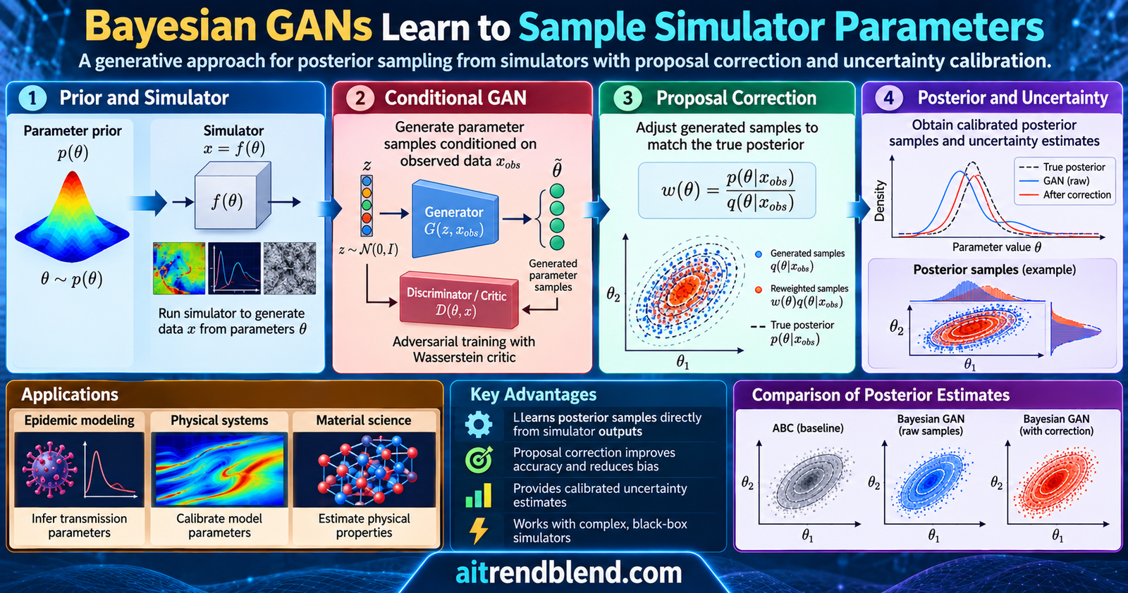
Wang and Ročková keep the simulation table but change what happens afterward. They learn a conditional sampler from the table. Instead of filtering a large bank of candidate draws anew for every observed dataset, a trained generator maps fresh noise and the dataset into parameter draws. This is an approximation to inference, with its own training cost and failure modes.
The change from generating data to generating explanations
The original GAN framework of Goodfellow and colleagues learns a generator by opposing it with a discriminator. For background, our explanation of how GANs work follows that mechanism. Here the generated object is a parameter vector that might explain observations under a simulator.
That change is easy to miss. A conventional data generator answers what another observation might look like. The Bayesian generator answers what the underlying settings might be, given an observation. The network is not learning a probability distribution over its own weights. The paper explicitly distinguishes its use of the term Bayesian GAN from approaches that put priors on GAN network parameters.
Training begins with pairs of parameters and simulated datasets. Each parameter vector is drawn from the prior, and the simulator produces the accompanying data. This table contains the joint relationship that inference needs. It includes examples of how different settings produce different observations, including the ambiguity that randomness introduces.
Equation 2. Real pairs come from simulation, and generated pairs keep the same conditioning data.
The critic sees two kinds of pair. One contains the actual parameter used to generate a simulated dataset. The other contains a parameter invented by the generator for that same dataset. Keeping the conditioning data unchanged is essential. It prevents the generator from winning simply by changing which datasets appear in its pairs.
At an ideal solution, the generated joint distribution matches the simulated joint distribution. Because both share the data marginal, matching the joint also matches the conditional parameter distribution. In finite training, limited network capacity and incomplete optimization intervene. The population argument explains the target. It does not certify a particular trained network.
Inside the conditional sampler and critic
The sampler takes two inputs, noise and a representation of the data. Noise gives it the freedom to return many possible parameter vectors for the same conditioning dataset. A model that ignores this input could produce a narrow collection of similar answers even when the true posterior has substantial uncertainty.
The critic receives a parameter vector and the conditioning data and returns a real score. It does not need a sigmoid probability for the Wasserstein training used in the main implementation. The two networks learn a conditional relationship by contrasting the simulated and generated pairs, rather than by regressing every dataset to a single parameter estimate.
For the Gaussian example, Appendix E describes three hidden layers of width 128 in both networks for the base method. The local refinements use two hidden layers of width 256. Noise dimension equals parameter dimension in that setup. The authors also explore ReLU and leaky ReLU activations and report no significant advantage of one over the other there.
Those choices are part of the experimental recipe, not universal instructions for simulator inference. A short vector of summaries and a long time series present very different learning problems. A practitioner should first decide what information the data representation retains, then choose an architecture that can handle that representation without discarding the structure of the simulator.
The wider context appears in our article on GAN mathematics and training dynamics and the Generative and Diffusion Models archive. This paper’s distinctive angle is conditional posterior sampling, including the consequences of changing the simulation proposal.
The loss and the constraint that make the game work
The paper writes its Wasserstein game with generated scores minus simulated scores inside a maximization over critics. Readers familiar with the reverse sign convention should pause here. Both conventions can describe an adversarial game when generator and critic signs are changed consistently. Mixing them in code changes the optimization.
Equation 3. The normalized form of Equation 5 retains the paper’s sign convention.
The critic must satisfy a Lipschitz restriction in the parameter argument. In practice the authors use a gradient penalty. They interpolate between a simulated parameter and a generated parameter while holding the conditioning dataset fixed. The gradient is taken with respect to that interpolated parameter, not a concatenated vector that also changes the data.
Equation 4. The penalty from Appendix E.1 discourages parameter gradients whose norm exceeds one.
This is a penalty from one side. Gradients below one are not forced upward toward one. That differs from the familiar penalty in Gulrajani and colleagues’ Wasserstein GAN training paper, which the source paper discusses. Replacing the penalty with a convenient standard implementation would change this detail.
Appendix E.2 gives 15 critic updates per generator update, a penalty coefficient of 5 and learning rates of one ten thousandth for the Gaussian base experiment. The practical purpose is to keep the critic informative while the generator changes. A training loss can be monitored, but posterior diagnostics remain necessary because an adversarial objective is not a direct certificate of uncertainty calibration.
Once trained, the generator draws independent noise and transforms it into samples from its learned approximation. Independent draws reduce dependence between samples. They do not remove approximation bias or prove that missing posterior modes have been recovered.
Why the second round needs a correction
A global sampler learns across datasets produced by the prior. That can be wasteful when the observed dataset occupies a small part of the prior predictive distribution. Many training pairs may teach the network about parameter regions that contribute little to the posterior for the observation that actually matters.
The second round begins with a pilot sampler conditioned on the observed data. Draw parameters from that pilot and simulate fresh datasets under them. This concentrates the new reference table around parameters already considered plausible. A new conditional sampler is trained on the table, with the aim of improving local reconstruction.
There is a statistical cost to this convenience. The parameters now come from the pilot proposal instead of the original prior. Without a correction, the refined conditional distribution targets the posterior associated with that proposal. A visually sharper density is not automatically the original Bayesian answer.
Equation 5. Importance correction returns proposal based draws toward the original prior target, subject to approximation error and adequate proposal support.
The proposal is itself implicit, so its density need not be available. The paper offers two estimation routes. With a tractable prior and a small parameter dimension, estimate the proposal density with a kernel estimator. Otherwise train a classifier to separate prior draws from proposal draws and use its estimated odds as a density ratio.
That classifier construction requires attention to the class sampling proportions. With equal class proportions, the estimated odds represent the prior to proposal ratio in the desired direction. Reversing labels reverses the correction. Unequal proportions need an adjustment. Neither a well behaved classification loss nor a smooth density plot proves that the estimated ratios are accurate.
Our practical reading is to examine effective sample size and the concentration of normalized weights. If a few draws carry nearly all the weight, the correction may be numerically fragile. Also inspect proposal support. No finite reweighting can restore a parameter region that the proposal never reaches. These are diagnostic recommendations, not additional performance results reported by the authors.
The variational refinement adds a local push
The second refinement uses the observed dataset inside the generator’s training loss. Alongside the global adversarial term, it evaluates generated parameters under the observed condition and adds a local critic term. The authors motivate this through implicit variational Bayes and the role of learned density ratios.
Equation 6. A normalized version of Equation 14. The relative coefficient must account for the chosen global and local sample counts.
The distinction between motivation and exact computation matters. A general Wasserstein critic is not automatically an exact log density ratio. The practical local score in this algorithm should not be described as an exactly evaluated evidence lower bound. It is a regularized adversarial objective designed to balance global learning with local adaptation.
Algorithm 3 also uses the pilot proposal to construct its reference table and retains importance correction at the output stage. The local term does not cancel the changed prior by itself. Treating the variational label as permission to drop the weights would omit a step explicitly present in the algorithm.
“The performance, however, is not uniformly better than Algorithm 2.”Wang and Ročková, Section 3, discussing the variational refinement
The authors observe spikier variational reconstructions in one Gaussian repetition and larger discrepancies than the other refinement. That is valuable evidence about the tradeoff. A stronger local push can improve some parameter estimates while producing an approximation whose shape is less faithful overall.
When the data are a set rather than a long vector
Flattening every observation into a single vector is a simple starting point. It becomes awkward when the number of observations grows. Network inputs become larger, memory requirements increase and the posterior can concentrate in a region that a broad prior table scarcely covers. The paper treats these as distinct problems rather than one generic scaling issue.
For independent and identically distributed observations, reordering the records should not change the posterior. The authors use the Deep Sets architecture of Zaheer and colleagues to build that invariance into both networks. The generator’s observation features depend on noise, and the critic’s observation features depend on the candidate parameter.
Equation 7. The pooled forms in Section 2.5 preserve observation order invariance for exchangeable inputs.
In the queueing demonstration, each observation contains the first five interdeparture times, and the authors consider 50, 100 and 200 independent observation vectors. With fixed network complexity, the set representation remains informative at the largest setting where simple stacking fails. The sequential batch approach also fails at the largest setting in the displayed experiment.
This is an architecture result with boundaries. Sum pooling reduces the growth of network input size, but it does not erase the cost of simulating, storing and processing more records. Nor should it be applied to an ordered time series as though every timestamp were exchangeable. Invariance is helpful only when it matches the statistical structure of the observations.
What the experiments establish
The study examines a Gaussian toy problem, a queueing example, a predator and prey process, a boom and bust process, and the historical outbreak application. These are different tests of an inference mechanism. They do not constitute a broad real world benchmark across simulator families, parameter dimensions and observation conditions.
The Gaussian example is useful because a reference posterior can be calculated from the exact likelihood. It uses four observations, each with two dimensions, and a parameter vector with five dimensions. Two parameter signs are not identifiable from the likelihood. The example therefore tests whether a sampler can retain multiple plausible regions rather than merely find one attractive point.
In that example, the authors compare maximum mean discrepancies using 1,000 posterior draws and ten repetitions. The refinement based on a second simulation round gives the smallest discrepancy in the plotted comparison. That supports the local proposal idea in this setting. It does not establish that the same variant wins for every simulator.
Population dynamics and the meaning of narrow intervals
The predator and prey experiment records 201 time points for each of two populations, with one trajectory used in the main setting. The GAN methods use summary statistics because the authors found them better empirically than directly using the time series. This is a reminder that representation choices remain important even when a method can accept raw data in principle.
The boom and bust example observes 250 time steps after 50 burn steps. Again, the reported network works on summaries. The comparison includes sequential neural likelihood, summary based ABC and Wasserstein ABC. Table 2 reports averages over ten repetitions, giving a more useful picture than a single posterior plot.
| Quantity | Base GAN | Second round | Variational refinement | Sequential neural likelihood |
|---|---|---|---|---|
| Growth rate r mean bias | 0.044 | 0.026 | 0.024 | 0.024 |
| Growth rate r credible interval width | 0.165 | 0.081 | 0.076 | 0.093 |
| Growth rate r coverage | 1.00 | 0.90 | 0.90 | 1.00 |
| Capacity parameter κ mean bias | 3.03 | 1.42 | 1.56 | 1.52 |
| Arrival rate β credible interval width | 0.39 | 0.24 | 0.23 | 0.39 |
| Arrival rate β coverage | 0.90 | 0.70 | 0.80 | 0.90 |
The source table labels the second round method B GAN RL, while Algorithms 2 and the surrounding discussion use the second step terminology. The table above refers to that refinement by its role. Scaled rows have been multiplied by the factors printed in the source table. Entries for coverage follow the table’s convention that coverage is one unless otherwise stated.
The interpretation is more interesting than a simple win count. Both refinements reduce the growth rate bias and interval width, but the coverage for that rate falls to nine out of ten repetitions. For the arrival rate, the second round’s narrow interval covers the truth in seven out of ten repetitions. Sharper uncertainty is not necessarily better calibrated uncertainty.
Ten repetitions also make the coverage estimate coarse. One different outcome changes the observed fraction by one tenth. The paper’s results justify optimism about localization and concern about calibration at the same time. They do not justify treating small differences between reported coverage fractions as precise population level conclusions.
The epidemic example and the clinical translation gap
The real data application uses 21 daily infected and recovered counts from the Tristan da Cunha common cold outbreak. The model includes a latent compartment for people infected but not yet infectious. Four quantities are estimated, the transmission rate, recovery rate, latent transition rate and the initial susceptible population, which the observations do not directly provide.
The paper simulates 100 datasets from each fitted posterior predictive distribution and compares them with the observed series. The authors report that all methods cover the observations and that the variational version gives the best fit in the plotted comparison. They also find multimodal posteriors for the recovery and latent transition rates.
These are valuable model fitting checks, but they are not clinical validation. One historical outbreak cannot show performance across contemporary populations, surveillance systems or changing disease dynamics. Agreement with the fitted series also does not establish prospective forecasting skill on unseen days. The paper provides no clinical accuracy endpoint or patient treatment comparison.
A clinical translation study would need an appropriate observation model, checks for missing and biased reporting, external datasets and a carefully defined decision task. Those are our proposed validation needs, not completed experiments. The authors explicitly leave model misspecification for future work, which is particularly relevant when a simulator is applied to human populations.
What the theorem promises and what it assumes
The theoretical target is a typical squared total variation distance between the true posterior and the learned approximation. Typical means the error is averaged over training randomness and considered under the data generating process. It does not mean a uniform guarantee for every possible observed dataset or every adversarial training trajectory.
Theorem 1 separates several contributors to the bound. The critic class must approximate relevant log density ratio functions. The generator class must approximate the conditional posterior family. The finite reference table introduces a complexity term involving the network classes’ pseudo dimensions. A prior concentration condition is also required.
Corollary 6 establishes that suitable network architectures and simulation table sizes can make the typical squared error vanish under its assumptions as observation dimensionality grows with fixed parameter dimension. It includes a realizability assumption and specified network classes. This is an existence and approximation result, not evidence that any convenient architecture trained by Adam will reach the required solution.
The gradient penalty used in practice also does not by itself certify all the boundedness and approximation conditions in the proof. Keep the theoretical network classes, the population optimization and the actual finite training run separate. The paper gives a principled way to understand error sources, which is already useful without turning its theorem into a training guarantee.
The theory identifies what has to improve. The experiments show that the strategy can improve selected approximations. A practitioner still needs to check posterior modes, weight stability, predictive fit and calibration for the simulator being used.
Limitations that should travel with the result
The sampler learns under the simulator and prior supplied to it. If the observed data do not fit that model, a sophisticated sampler may return a precise answer to the wrong inferential question. The authors identify misspecification as a future direction. Faster sampling does not repair a mistaken model or a missing source of observational noise.
The useful second round depends on the pilot. If the pilot overlooks a mode, the localized simulation table may reinforce that omission. Kernel proposal estimation becomes more difficult in larger parameter dimensions, while classifier ratio estimates require their own diagnostics. These dependencies are part of the method, not minor postprocessing details.
The comparison with sequential neural likelihood is informative but limited to the configurations studied. Summary selection, prior bounds, simulation budgets and stopping choices affect results. The paper’s favorable examples should guide further testing rather than replace it. No single displayed benchmark establishes a universal advantage for an implicit generator over a density based model.
Timing requires special care. Table 5 uses CPUs for the ABC and sequential likelihood comparators and GPUs for the GAN methods. The refinement timings omit the pilot run. Those are useful reported operating costs, but they do not support an unqualified claim of faster complete inference on matched hardware.
The health example has especially narrow evidence. It uses one 21 day outbreak series, with no external clinical cohort and no prospective deployment. Reported multimodality suggests that some parameter combinations remain difficult to distinguish. It would be inappropriate to turn those posteriors into medical recommendations or public health decisions without task specific validation and qualified oversight.
Where this leaves simulator inference
The core achievement is a conditional generator that approximates a Bayesian posterior through simulation and adversarial learning. It avoids needing an explicit likelihood or an explicitly evaluable posterior density for the base sampling step. Once learned, the map can transform independent noise into draws for a fixed observed dataset.
The conceptual change is to spend simulation effort on learning an inference map. That map can be reused across observations under the same model and data representation. The local variants then spend additional effort around a particular observation. Their correction steps show why computational convenience has to remain tied to the statistical target.
The idea can travel to ecology, queueing and other settings where simulation is feasible and uncertainty matters. The application should be chosen according to the simulator’s credibility and the information in the observations. A neural generator is most useful when those foundations are clear enough to make posterior approximation meaningful.
The remaining limits are substantial. Adversarial training can be unstable, proposals can miss important regions and narrow intervals can have poor coverage. The reported experiments include improvements and exceptions. That mixture is more useful than a universal claim because it tells readers which parts need checking in their own implementation.
Future work should examine calibration across more datasets, proposal robustness, model misspecification and matched computing budgets. The paper also points toward architectures that reflect exchangeability and other statistical structure. Better representations may reduce the burden of learning, but they must preserve the information that the inference task depends on.
The most persuasive promise is a faster way to explore uncertainty, supported by diagnostics that make that uncertainty worth trusting.
PyTorch reference implementation
The complete listing below is editorial code following Algorithms 1 to 3 and the optional set construction in Section 2.5. It includes both proposal correction routes, training, weighted evaluation and a runnable smoke test on artificial Gaussian data. It is not the authors’ implementation and does not reproduce their experimental tables.
Several departures are intentional. Appendix E reports all weights initialized at zero, which can leave a multilayer ReLU network without useful hidden gradients. This listing uses random weight initialization. It also omits dropout so the generator is a deterministic map for fixed noise and data, and uses a tiny demonstration budget. Those choices must be reported if the code is extended into an experiment.
The code passed a Python syntax check here. PyTorch was not installed in this execution environment, so the included smoke test has not been run here. Its assertions check numerical mechanics and set order invariance. They do not establish posterior accuracy. Use a supported PyTorch installation, run the smoke test first, then replace the simulator, prior and evaluation design for your application.
"""Editorial B-GAN reference implementation for Wang and Rockova (JMLR 2026).
Requires Python 3.10+ and PyTorch. No external datasets are downloaded.
Implements Algorithms 1-3, Eq. 39, and optional Section 2.5 Deep Sets.
This is not the authors' software or a reproduction of their benchmark tables.
Departures: random initialization instead of the reported all-zero initialization;
no dropout, to keep g(z,x) deterministic; tiny Gaussian smoke data and budget.
The VB local critic term follows Eq. 14; it is not an exact KL/ELBO evaluator.
"""
from dataclasses import dataclass
from typing import Callable
import copy
import math
import torch
from torch import nn
from torch.nn import functional as F


def mlp(inp, hidden, out):
    layers = []
    for width in hidden:
        layers.extend((nn.Linear(inp, width), nn.ReLU()))
        inp = width
    layers.append(nn.Linear(inp, out))
    net = nn.Sequential(*layers)
    for layer in net:
        if isinstance(layer, nn.Linear):
            nn.init.xavier_uniform_(layer.weight)
            nn.init.zeros_(layer.bias)
    return net


class ConditionalMap(nn.Module):
    """Dense conditioning, or sum pooling with per-item latent conditioning."""
    def __init__(self, xdim, latent_dim, outdim, hidden, set_input=False):
        super().__init__()
        self.set_input = set_input
        if set_input:
            self.phi = mlp(xdim + latent_dim, hidden[:1], hidden[0])
            self.rho = mlp(hidden[0] + latent_dim, hidden, outdim)
        else:
            self.rho = mlp(xdim + latent_dim, hidden, outdim)

    def forward(self, latent, x):
        if self.set_input:
            if x.ndim != 3:
                raise ValueError('Set data require [batch, observations, features].')
            repeated = latent[:, None, :].expand(-1, x.size(1), -1)
            pooled = self.phi(torch.cat((repeated, x), -1)).sum(1)
            features = torch.cat((latent, pooled), -1)
        else:
            if x.ndim != 2:
                raise ValueError('Dense data require [batch, flattened features].')
            features = torch.cat((latent, x), -1)
        return self.rho(features)


class BGAN(nn.Module):
    def __init__(self, xdim, theta_dim, hidden=(128, 128, 128), set_input=False):
        super().__init__()
        self.theta_dim = theta_dim
        self.generator = ConditionalMap(xdim, theta_dim, theta_dim, hidden, set_input)
        self.critic = ConditionalMap(xdim, theta_dim, 1, hidden, set_input)

    def noise(self, count):
        p = next(self.parameters())
        return torch.randn(count, self.theta_dim, device=p.device, dtype=p.dtype)

    def score(self, theta, x):
        return self.critic(theta, x).squeeze(-1)

    @torch.no_grad()
    def sample(self, x0, count):
        was_training = self.training
        self.eval()
        x = x0.unsqueeze(0).expand(count, *x0.shape)
        out = self.generator(self.noise(count), x)
        self.train(was_training)
        return out


def one_sided_penalty(model, theta, fake, x):
    """Eq. 39. Differentiate in theta only; do not interpolate x."""
    epsilon = torch.rand(theta.size(0), 1, device=theta.device)
    mixed = (epsilon * theta + (1 - epsilon) * fake.detach()).requires_grad_(True)
    score = model.score(mixed, x)
    gradient = torch.autograd.grad(score.sum(), mixed, create_graph=True)[0]
    return F.relu(gradient.norm(2, dim=1) - 1).square().mean()


@dataclass
class Config:
    steps: int = 1000  # Generator updates, not passes over the whole reference table.
    batch: int = 1280
    ncritic: int = 15
    lr: float = 1e-4
    gp_weight: float = 5.0
    vb_weight: float = 0.0  # Separate coefficient from the gradient penalty.


def train(model, theta, x, cfg, x0=None):
    """Paper sign convention: critic maximizes fake-real, generator minimizes fake.
    Critic minimization is therefore real-fake+penalty. Matching batch counts
    for global and local terms keeps mean losses proportional to Eq. 14 sums.
    """
    if cfg.steps < 1 or cfg.batch < 1 or cfg.ncritic < 1:
        raise ValueError('Positive steps, batch and ncritic are required.')
    if cfg.gp_weight < 0 or cfg.vb_weight < 0:
        raise ValueError('Loss coefficients must be nonnegative.')
    if len(theta) != len(x) or len(theta) < 2:
        raise ValueError('Reference table pairs must align and contain at least two rows.')
    if not torch.isfinite(theta).all() or not torch.isfinite(x).all():
        raise ValueError('Reference data must be finite.')
    if cfg.vb_weight and x0 is None:
        raise ValueError('Observed x0 is required for VB refinement.')
    opt_c = torch.optim.Adam(model.critic.parameters(), lr=cfg.lr)
    opt_g = torch.optim.Adam(model.generator.parameters(), lr=cfg.lr)
    history = []
    model.train()
    for step in range(cfg.steps):
        for _ in range(cfg.ncritic):
            ix = torch.randint(len(theta), (cfg.batch,), device=theta.device)
            tb, xb = theta[ix], x[ix]
            with torch.no_grad():
                fake = model.generator(model.noise(cfg.batch), xb)
            penalty = one_sided_penalty(model, tb, fake, xb)
            c_loss = model.score(tb, xb).mean() - model.score(fake, xb).mean()
            c_loss = c_loss + cfg.gp_weight * penalty
            if not torch.isfinite(c_loss):
                raise RuntimeError('Nonfinite critic loss.')
            opt_c.zero_grad(set_to_none=True)
            c_loss.backward()
            opt_c.step()
        ix = torch.randint(len(theta), (cfg.batch,), device=theta.device)
        xb = x[ix]
        for p in model.critic.parameters():
            p.requires_grad_(False)
        try:
            fake = model.generator(model.noise(cfg.batch), xb)
            g_loss = model.score(fake, xb).mean()
            if cfg.vb_weight:
                observed = x0.unsqueeze(0).expand(cfg.batch, *x0.shape)
                local = model.generator(model.noise(cfg.batch), observed)
                g_loss = g_loss + cfg.vb_weight * model.score(local, observed).mean()
            if not torch.isfinite(g_loss):
                raise RuntimeError('Nonfinite generator loss.')
            opt_g.zero_grad(set_to_none=True)
            g_loss.backward()
            opt_g.step()
        finally:
            for p in model.critic.parameters():
                p.requires_grad_(True)
        history.append((float(c_loss.detach()), float(g_loss.detach())))
    return history


@torch.no_grad()
def make_reference(prior_sample: Callable, simulate: Callable, count):
    theta = prior_sample(count)
    x = simulate(theta)
    if theta.ndim != 2 or len(x) != count:
        raise ValueError('Simulator and prior must preserve the batch dimension.')
    return theta, x


class DiagonalKDE:
    """Low-dimensional pilot proposal density estimator for Eq. 7.
    Scott bandwidth is an editorial choice. KDE tails and support need diagnosis.
    Chunking bounds temporary memory; no arbitrary weight clipping is used.
    """
    def __init__(self, samples):
        if len(samples) < 2 or samples.ndim != 2:
            raise ValueError('KDE requires at least two parameter samples.')
        self.samples = samples.detach().clone()
        n, d = samples.shape
        self.bandwidth = samples.std(0).clamp_min(1e-4) * n ** (-1 / (d + 4))

    @torch.no_grad()
    def log_prob(self, query, chunk=128):
        n, d = self.samples.shape
        normalizer = self.bandwidth.log().sum() + 0.5 * d * math.log(2 * math.pi)
        output = []
        for q in query.split(chunk):
            residual = (q[:, None, :] - self.samples[None, :, :]) / self.bandwidth
            log_kernel = -0.5 * residual.square().sum(-1) - normalizer
            output.append(torch.logsumexp(log_kernel, 1) - math.log(n))
        return torch.cat(output)


class PriorProposalClassifier(nn.Module):
    """Optional Eq. 8 route for an implicit prior. Prior=1, proposal=0.
    Equal class sizes are essential for the logit to estimate log prior/proposal.
    This estimator needs calibration checks; a low loss alone is not validation.
    """
    def __init__(self, dim):
        super().__init__()
        self.net = mlp(dim, (64, 64), 1)

    def forward(self, theta):
        return self.net(theta).squeeze(-1)

    def fit(self, prior, proposal, steps=200, batch=128, lr=1e-3):
        opt = torch.optim.Adam(self.parameters(), lr=lr)
        for _ in range(steps):
            a = prior[torch.randint(len(prior), (batch,), device=prior.device)]
            b = proposal[torch.randint(len(proposal), (batch,), device=proposal.device)]
            logits = self(torch.cat((a, b)))
            labels = torch.cat((torch.ones(batch, device=a.device), torch.zeros(batch, device=b.device)))
            loss = F.binary_cross_entropy_with_logits(logits, labels)
            opt.zero_grad(set_to_none=True)
            loss.backward()
            opt.step()
        return self


@torch.no_grad()
def importance_weights(samples, prior_log_prob=None, proposal_kde=None, classifier=None):
    if classifier is not None:
        log_ratio = classifier(samples)  # logit D = log prior/proposal with equal classes.
    elif prior_log_prob is not None and proposal_kde is not None:
        log_ratio = prior_log_prob(samples) - proposal_kde.log_prob(samples)
    else:
        raise ValueError('Supply a classifier or both prior density and proposal KDE.')
    if torch.isnan(log_ratio).any() or torch.isposinf(log_ratio).any() or not torch.isfinite(log_ratio).any():
        raise RuntimeError('Importance ratios cannot be normalized. Check proposal support.')
    weights = torch.softmax(log_ratio, 0)
    return weights


def refine(pilot, x0, simulate, count, cfg, hidden=(256, 256)):
    """Algorithm 2 when vb_weight=0, Algorithm 3 when vb_weight>0.
    Returns the refined sampler and KDE of the PILOT proposal, not refined output.
    Both variants require original-prior importance correction after sampling.
    """
    theta = pilot.sample(x0, count)
    with torch.no_grad():
        x = simulate(theta)
    proposal = DiagonalKDE(pilot.sample(x0, max(256, count)))
    set_input = pilot.generator.set_input
    xdim = x.shape[-1]
    refined = BGAN(xdim, pilot.theta_dim, hidden, set_input).to(theta.device)
    history = train(refined, theta, x, cfg, x0 if cfg.vb_weight else None)
    return refined, proposal, history


@torch.no_grad()
def evaluate(samples, weights=None, reference=None, true_theta=None):
    """Weighted moments, 95% equal-tail intervals, ESS and optional reference MMD.
    One-case truth containment is NOT repeated-data coverage.
    MMD uses a fixed RBF bandwidth of 1 for this demo, not the paper benchmark.
    """
    n = len(samples)
    weights = torch.full((n,), 1 / n, device=samples.device) if weights is None else weights
    if (weights < 0).any() or not torch.isfinite(weights).all() or weights.sum() <= 0:
        raise ValueError('Finite nonnegative weights with positive total are required.')
    weights = weights / weights.sum()
    mean = (samples * weights[:, None]).sum(0)
    var = ((samples - mean).square() * weights[:, None]).sum(0)
    lower, upper = [], []
    for j in range(samples.size(1)):
        values, order = samples[:, j].sort()
        cumulative = weights[order].cumsum(0)
        low = torch.searchsorted(cumulative, torch.tensor(0.025, device=samples.device)).clamp_max(n-1)
        high = torch.searchsorted(cumulative, torch.tensor(0.975, device=samples.device)).clamp_max(n-1)
        lower.append(values[low]); upper.append(values[high])
    lower, upper = torch.stack(lower), torch.stack(upper)
    result = {'mean': mean, 'variance': var, 'lower95': lower, 'upper95': upper,
              'ess': 1 / weights.square().sum()}
    if true_theta is not None:
        result['contains_truth'] = (lower <= true_theta) & (true_theta <= upper)
    if reference is not None:
        # Biased weighted MMD^2 includes diagonals and is nonnegative in theory.
        if len(samples) > 2048 or len(reference) > 2048:
            raise ValueError('Use a subsample for quadratic-memory MMD.')
        kernel = lambda a, b: torch.exp(-0.5 * torch.cdist(a, b).square())
        kxx, kyy, kxy = kernel(samples, samples), kernel(reference, reference), kernel(samples, reference)
        result['mmd2'] = (weights @ kxx @ weights + kyy.mean() - 2 * (weights[:, None] * kxy).sum() / len(reference)).clamp_min(0)
    return result


def smoke_test():
    """Executes all three training paths, correction routes and set invariance.
    Tiny budgets verify mechanics only; posterior accuracy is not asserted.
    """
    torch.manual_seed(42)
    torch.set_num_threads(1)
    count, observations = 128, 4
    prior = lambda n: torch.randn(n, 1)
    simulate = lambda theta: theta + torch.randn(len(theta), observations)
    log_prior = lambda theta: (-0.5 * theta.square() - 0.5 * math.log(2 * math.pi)).sum(-1)
    theta, x = make_reference(prior, simulate, count)
    x0 = torch.tensor([0.2, 0.6, 0.4, 0.0])
    cfg = Config(steps=3, batch=16, ncritic=2)
    pilot = BGAN(observations, 1, hidden=(16, 16))
    train(pilot, theta, x, cfg)
    # Known conjugate posterior for editorial Gaussian test, not a paper experiment.
    variance = 1 / (1 + observations)
    mean = x0.sum() / (1 + observations)
    exact = mean + math.sqrt(variance) * torch.randn(128, 1)
    for local_weight in (0.0, 0.1):
        local_cfg = copy.copy(cfg)
        local_cfg.vb_weight = local_weight
        refined, proposal, history = refine(pilot, x0, simulate, count, local_cfg, hidden=(16, 16))
        draws = refined.sample(x0, 64)
        weights = importance_weights(draws, log_prior, proposal)
        summary = evaluate(draws, weights, reference=exact)
        assert torch.isfinite(draws).all() and torch.isfinite(summary['ess'])
        assert torch.allclose(weights.sum(), torch.tensor(1.0), atol=1e-6)
        print('VB weight', local_weight, 'ESS', float(summary['ess']), 'MMD2', float(summary['mmd2']))
    classifier = PriorProposalClassifier(1).fit(prior(128), pilot.sample(x0, 128), steps=2, batch=16)
    ratio_weights = importance_weights(pilot.sample(x0, 32), classifier=classifier)
    assert torch.isfinite(ratio_weights).all()
    sets = BGAN(1, 1, hidden=(16, 16), set_input=True)
    set_x = x[:8, :, None]
    z = sets.noise(8)
    permutation = torch.tensor([3, 0, 2, 1])
    assert torch.allclose(sets.generator(z, set_x), sets.generator(z, set_x[:, permutation]), atol=1e-5)
    assert torch.allclose(sets.score(theta[:8], set_x), sets.score(theta[:8], set_x[:, permutation]), atol=1e-5)
    train(sets, theta, x[:, :, None], Config(steps=1, batch=8, ncritic=1))
    print('Smoke checks completed. This is not evidence of posterior convergence.')


if __name__ == '__main__':
    smoke_test()
Frequently asked questions
What does a Bayesian GAN generate?
It generates parameter draws conditional on observations under a simulator and prior. It approximates the posterior rather than simply producing new observations.
Does the method require an evaluable likelihood?
The base sampler requires simulated parameter and data pairs, not an evaluable likelihood. Proposal correction in the refinements requires a density ratio estimate.
Why must the second simulation round use importance weights?
Its reference table uses a pilot proposal instead of the original prior. The weights correct for that change, subject to estimation error and adequate proposal support.
Does the variational refinement always perform better?
No. The paper reports improvements in some settings and spikier approximations in another Gaussian repetition. Posterior shape and calibration need separate checks.
Does the outbreak experiment establish clinical usefulness?
No. It fits one historical outbreak series and checks posterior predictive simulations. It does not provide external clinical validation, treatment evidence or prospective deployment results.
Has the included PyTorch code reproduced the paper?
No. It is an editorial reference implementation with a small artificial smoke test. It passed a syntax check here, but the smoke test was not run because PyTorch was unavailable.
Read the paper before adapting the sampler
The source contains the proofs, full posterior plots, algorithm details and the historical outbreak observations.
Read the JMLR paperSee the outbreak data in Table 3Wang, Y., and Ročková, V. (2026). Generative Bayesian Inference with GANs. Journal of Machine Learning Research, 27(29), pages 1 to 48. Official publication record.
This analysis is based on the published paper and an independent evaluation of its claims.