What is LazyDINO in one sentence?

It is a method for Bayesian inverse problems with expensive simulators that builds a neural surrogate offline from simulator outputs and derivatives, and then fits a low dimensional transport map to the posterior for each new data set using only that surrogate.

It is a transport map that bends the prior only inside a small latent subspace and leaves every other direction equal to the prior. The subspace is chosen so that it holds the directions in which the data change the prior the most.

Why does the surrogate need to match derivatives and not only outputs?

The online optimization follows gradients of the surrogate objective, so errors in the surrogate's slopes steer the transport map in the wrong direction. The paper proves a bound in which the Jacobian error appears next to the output error, and the derivative informed loss minimizes exactly that quantity.

Does LazyDINO beat the Laplace approximation?

In most reported metrics it does, with fewer than 1,000 offline simulator evaluations, and it keeps improving when the posterior is not Gaussian. In the first example, however, the Laplace approximation kept the lower covariance error, and the authors report that.

What does the method require from my simulator?

It needs outputs and Jacobian samples, usually through forward or adjoint sensitivity solves, and a Gaussian prior in the formulation the paper gives. It pays off most when many data sets share the same simulator and prior.

Is the code in this article the authors' code?

No. The listing is a small editorial sketch on a one dimensional PDE meant to show how the pieces fit together. The authors' implementation and numerical examples are in their public dinox repository.

LazyDINO Amortizes Bayesian Inversion for PDE Models

Analysis by the aitrendblend editorial team · Based on Cao, Chen, Brennan, O’Leary-Roseberry, Marzouk and Ghattas, JMLR 27 (2026) · 5 October 2026

Bayesian inverse problems
transport maps
lazy maps
derivative informed learning
neural operators
amortized inference

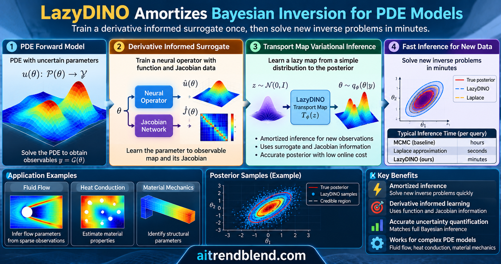
LazyDINO workflow with an offline derivative informed surrogate and an online lazy transport map for Bayesian inversion of a PDE model, from the 2026 JMLR paper by Cao, Chen, Brennan, O'Leary-Roseberry, Marzouk and Ghattas — Feature illustration. The expensive simulations happen once offline, and each new data set only touches a cheap surrogate.

Picture a thin film clamped in a tensile tester and stretched until it is visibly longer. About sixty displacement readings come off the sensors, and the question is where the film is stiff and where it is soft. Answering that properly means a probability distribution over a stiffness field with thousands of unknowns, and every candidate field needs a nonlinear finite element solve to check. A new JMLR paper shows how to pay for those solves once, ahead of time, and then answer each new set of readings with a short optimization that never touches the simulator again. In the authors’ second example the online step took about twelve and a half minutes of transport map training per data set, in a benchmark run the authors say can be stopped much earlier.

Key points

LazyDINO splits Bayesian inversion into an offline phase, which builds a neural surrogate of the simulator from samples of its outputs and its derivatives, and an online phase, which fits a transport map to the posterior for each new data set using only the surrogate.
The surrogate and the transport map live in the same low dimensional subspace, found from Jacobian samples, so training cost does not grow with the number of discretized parameters.
Theory in the paper says the surrogate’s Jacobian error, and not only its output error, controls how well the online optimization behaves. That is the justification for training with derivative data.
On two PDE examples with about 1,700 and 2,100 discretized parameters, the authors report one to two orders of magnitude less offline cost than two amortized baselines for the same posterior accuracy.
The Laplace approximation is not beaten everywhere. In the first example it keeps the lower covariance error, and the method needs Jacobian data, which not every simulator can supply cheaply.
We include a small PyTorch toy on a one dimensional PDE that shows the same ordering in miniature. It is our own sketch and not the authors’ code.

The problem the paper attacks

Inverse problems run physics backwards. A simulator takes a parameter, such as a stiffness or a diffusivity field, and predicts what sensors would read. The inverse problem observes noisy readings and asks which parameters could have produced them. The Bayesian version does not return a single answer. It returns a posterior distribution that says how plausible each parameter field is and how much the data actually pins down.

Lianghao Cao, Joshua Chen, Michael Brennan, Thomas O’Leary-Roseberry, Youssef Marzouk and Omar Ghattas, working across Caltech, Colorado State, MIT, Ohio State and the University of Texas at Austin, write the setting in the usual way. Data $y$ equal the parameter to observable map $G(m)$ plus Gaussian noise, and Bayes’ rule weighs the prior by the likelihood.

$$\frac{d\mu^y}{d\mu}(m)\ \propto\ \exp\Big(-\tfrac12\big\|\Gamma_n^{-1/2}\big(G(m)-y\big)\big\|^2\Big)$$

Equation 1. The posterior as a reweighting of the prior

Two things make this expensive. Every likelihood evaluation needs a full run of a nonlinear PDE solver, and the parameter $m$ is a field, so after discretization it has thousands of coordinates. Sampling methods that call the simulator millions of times are out of reach when each call takes seconds or minutes.

The authors care about a particular regime where this cost is repeated many times. A predictive digital twin sees a stream of fresh sensor data. Bayesian optimal experimental design scores many hypothetical data sets. In both, the simulator and the prior stay fixed while the data change, so it is natural to ask for amortization, meaning the heavy computation happens before the data arrive and each new posterior costs little. For a gentle introduction to why uncertainty estimates need care, see our explainer on better uncertainty from sparse Gaussian processes.

Lazy maps, a transport map that only works where the data speak

The method belongs to the family called transport map variational inference. It builds a map $T_\theta$ that pushes the prior forward into something close to the posterior, and it chooses the parameters $\theta$ by minimizing the reverse Kullback Leibler divergence, written rKL below. Once the map exists, posterior samples cost one map evaluation per sample, which is why the approach is attractive for fast repeated inference. Our look at stochastic transport for composite image restoration shows a neighboring use of transport ideas in imaging.

The difficulty is dimension. A map on thousands of coordinates needs thousands of variate functions, and flexible flows add layers until tuning becomes a chore. The paper builds on lazy maps from Brennan and coauthors (2020), which restrict the nonlinear part of the map to a small latent space and leave everything else alone.

$$T_\theta\ =\ D_r\circ\tau_\theta\circ E_r\ +\ \big(\mathrm{Id}_M-D_r\circ E_r\big)$$

Equation 2. A lazy map, with encoder $E_r$, decoder $D_r$ and latent map $\tau_\theta$

Read the formula from the outside in. The encoder $E_r$ squeezes a parameter field into $d_r$ numbers, the latent map $\tau_\theta$ bends those numbers to match the posterior, and the decoder puts the field back together. The second term is the identity on the leftover directions, so everything outside the latent space is simply the prior. The bet is that the data only update the prior along a few directions, which is plausible when the sensors are few and the physics smooths things out.

Choosing the subspace from derivatives

Which directions deserve the nonlinear treatment? The authors follow earlier work by Cui and Zahm (2021) and pick the directions in which the simulator output is most sensitive, averaged over the prior. Concretely they average the Gauss Newton Hessian of the data misfit and take its leading eigenvectors.

$$H_A=\mathbb{E}_{m\sim\mu}\big[DG(m)^*DG(m)\big],\qquad H_A\,\psi_j=\lambda_j\,\psi_j,\qquad E_r m=\big(\langle\psi_j,m\rangle\big)_{j\le d_r}$$

Equation 3. The derivative informed subspace from Jacobian samples

The word that matters is Jacobian. Building $H_A$ requires samples of the derivative of the simulator, obtained through forward or adjoint sensitivity solves. That demand shows up again later, because it is both the source of the method’s strength and its entry price. In the paper’s two examples the authors use $d_r=200$ and estimate the subspace from 1,000 Monte Carlo samples. They do not vary either number in the study, a point we return to under limitations.

Swap the simulator for a surrogate during the online step

Training the transport map by rKL minimization needs the simulator and its Jacobian at every optimization step, which is the bottleneck the paper wants to remove. The remedy is a ridge function surrogate that reuses the same latent space.

$$G(m)\ \approx\ V\,g_w\big(E_r m\big),\qquad \min_\theta\ \mathbb{E}_{z\sim\mathcal N(0,I_{d_r})}\Big[\tfrac12\big\|g_w(\tau_\theta(z))-V^*y\big\|^2+\tfrac12\|\tau_\theta(z)\|^2-\log\big|\det\nabla\tau_\theta(z)\big|\Big]$$

Equation 4. The reduced basis surrogate and the surrogate driven rKL objective

Here $g_w$ is a small neural network that eats the latent coordinates and outputs the whitened observables, and $V$ is a basis for the data space. Notice what the second formula contains. The simulator is gone. The only expensive object is a network evaluation, which a GPU can batch by the thousand. The authors call the surrogate architecture a reduced basis neural operator, and they use the version known as DIPNet from O’Leary-Roseberry and coauthors (2022).

Train on derivatives, not only on outputs

The second design choice is the loss. A standard fit, which the paper calls conventional or L2 training and abbreviates RB NO, asks the network to match simulator outputs. The paper’s recipe, abbreviated RB DINO in the paper and here, adds a term that asks the network to match the simulator’s Jacobian in the latent space as well.

$$\min_w\ \mathbb{E}_{m\sim\mu}\Big[\big\|V^*G(m)-g_w(E_rm)\big\|^2+\big\|V^*DG(m)D_r-\nabla g_w(E_rm)\big\|_F^2\Big]$$

Equation 5. Derivative informed training, a Sobolev style loss

Why spend training signal on derivatives? Because the optimizer in the online step follows gradients of the surrogate. A network can match outputs everywhere and still have slopes that point the wrong way, and the transport map then converges to the wrong place. The next section turns that intuition into a statement the paper proves.

Key takeaway

The same Jacobian samples do two jobs. They pick the low dimensional subspace where the posterior differs from the prior, and they teach the surrogate to have trustworthy slopes inside that subspace.

What the theory actually says

The paper has two theoretical results that matter in practice, and it is worth stating each with its caveats because they are easy to over read. Both bound the error caused by swapping the simulator for a surrogate.

Theorem 4 bounds the expected forward KL divergence between the true posterior and the posterior you would get if the surrogate replaced the simulator in the likelihood, averaged over the data distribution. The bound is a sum of two pieces.

$$\mathbb{E}_{y}\big[D_{\mathrm{KL}}(\mu^y\,\|\,\tilde\mu^y)\big]\ \le\ \underbrace{\mathrm{Tr}\big((\mathrm{Id}-P)H_A(\mathrm{Id}-P)\big)}_{\text{parameter reduction error}}\ +\ \underbrace{\text{latent representation error of }g_w}_{\text{how well the network fits}}$$

Equation 6. The structure of Theorem 4 (the exact norm in the second term is in the paper)

The first piece depends only on the subspace and is smallest when the subspace is the leading eigenspace of $H_A$. That is why the eigenproblem in Equation 3 is not a heuristic here, it minimizes the bound. The second piece is the plain output error of the network. Together they explain the DIPNet architecture, since the encoder from Jacobian samples is the minimizer of the first term.

Theorem 5 handles the part that Theorem 4 misses. The transport map comes out of a gradient based optimization, so closeness of the targets is not enough and the gradients of the objective must also agree. The theorem bounds the expected error of the surrogate objective gradient by a Sobolev norm of the surrogate error.

$$\mathbb{E}_y\big\|\nabla_\theta L^y-\nabla_\theta\tilde L^y\big\|\ \lesssim\ \Big(\mathbb{E}_{z}\Big[\big\|g_{\mathrm{opt}}-g_w\big\|^2+\big\|\nabla g_{\mathrm{opt}}-\nabla g_w\big\|_F^2\Big]\Big)^{1/2}$$

Equation 7. The gradient error bound of Theorem 5, which contains the Jacobian error

The right side is exactly the quantity that derivative informed training minimizes. Corollary 6 carries the same expression to the optimality gap, meaning how much worse the surrogate trained transport map is than the one trained on the true simulator. Its assumptions are stronger. The rKL objective must be locally strongly convex near its minimizers, and the surrogate’s minimizers must land inside those convex regions.

Table 1. The theoretical results and what each one licenses
Result	What it bounds	What it justifies	Main condition
Theorem 4	Expected forward KL between true and surrogate posteriors	The DIPNet architecture and the derivative based subspace	A projector built from an orthonormal reduced basis
Theorem 5	Expected error of the surrogate rKL gradient	Training with Jacobian data, since the bound contains the Jacobian error	Bounded density ratio and bounded parameter Jacobian of the transport map
Corollary 6	Expected optimality gap of the trained transport map	The same Sobolev style loss	Local strong convexity and surrogate minimizers inside the convex region

Two readings keep these results honest. They are upper bounds, so they say which error to control and not how large the final error will be. And the same Sobolev error appears in Theorem 5 and in the loss, which is a good sign of design coherence and not an independent confirmation that the loss is the best possible one. The authors do not claim optimality of the loss among all choices.

“by first building a reliable surrogate PtO map over the prior using a fixed number of samples, we can later enable an optimization algorithm requiring orders of magnitude more samples.”
Cao, Chen, Brennan, O’Leary-Roseberry, Marzouk and Ghattas, JMLR 27 (2026), on why the surrogate pays off

The offline and online phases side by side

Put the pieces together and the workflow has two stages. Offline, the authors sample parameters from the prior and run the simulator for the outputs, then run forward or adjoint sensitivity solves for the Jacobians. They compute the derivative subspace, then train the surrogate with the loss of Equation 5. Online, for each new data vector, they train a latent transport map against the cheap objective of Equation 4, which takes seconds to minutes, and then draw as many posterior samples as they like by evaluating the map. The same surrogate serves every later data set.

The main competitor in the paper is amortized simulation based inference, shortened here to ASBI. It trains a conditional normalizing flow offline on pairs of parameters and simulated data, with a forward KL objective, so that a single network maps any data vector to a posterior. At test time sampling needs the flow to be inverted. The table summarizes how the methods in the paper differ, drawing on the authors’ Table 2.

Table 2. How the compared methods spend their budget
Method	Offline data	Transport map training	Online simulator calls
LazyDINO	Simulator outputs and Jacobians, trained with the Sobolev style loss	Online, reverse KL against the surrogate	None
LazyNO	Simulator outputs only, trained with the L2 loss	Online, reverse KL against the surrogate	None
ASBI	Pairs of parameters and noisy simulated data	Offline, a conditional flow with forward KL, sampled by inversion	None
LazyMap	None	Online, reverse KL against the true simulator	Every optimization step
Laplace approximation	None	Not applicable, a Gaussian from the MAP point and the Hessian	For the MAP and Hessian

One structural advantage deserves a mention. LazyDINO builds a surrogate for the simulator and not for the likelihood, so the same surrogate handles many observations. The authors note that this extends to several independent data sets from the same experiment, since each contributes one block of a product likelihood. An ASBI network trained for one data format does not offer that for free.

What the experiments show

The study uses two PDE problems in two space dimensions, each with four synthetic observation sets drawn by sampling the prior, running the model and adding noise. The priors are Matérn Gaussian fields.

Table 3. The two inverse problems in the paper
Item	Example I	Example II
Physics	Nonlinear reaction diffusion with a cubic reaction term	Neo Hookean hyperelastic thin film under uniaxial stretch
Unknown field	Log diffusivity	Young’s modulus, ranging from 1 to 7 through an error function link
Grid and size	40 by 40 cells, 1,681 parameter and 3,362 state degrees of freedom	64 by 32 cells, 2,145 parameter and 16,770 state degrees of freedom
Observations	25 locally averaged points	64 values from 32 interior points
Signal to noise ratio	About 500	About 500

Both examples use the same network recipe. The surrogate is a multilayer perceptron with seven hidden layers of width 400 and GELU activations, and the transport map is an inverse autoregressive flow with 30 layers. The reference posterior comes from up to five million MCMC samples. Posterior quality is scored by relative errors in the mean, covariance and a low dimensional skewness, by a shifted rKL and fKL estimate, and by an effective sample size percentage from importance sampling called ANIS ESS.

Surrogate quality and cost

Before looking at posteriors, the authors compare the two surrogate training styles. In Example I the derivative informed surrogate is 64 times more cost efficient than the conventional one, meaning it reaches a given accuracy with 64 times fewer simulator evaluations by the authors’ measure. In Example II the gain is 8 to 32 times. Cost here counts nonlinear PDE solves, and the authors argue in their Remark 8 that Jacobian generation adds negligible extra cost with sparse direct solvers.

Posterior accuracy

On posterior moments the picture matches the abstract. Setting aside what the authors call a statistical anomaly at 500 samples, LazyDINO is 64 times more sample efficient than LazyNO for the mean in Example I, 4 times for the covariance, and 64 times for the skewness. Against ASBI the mean gain is also 64 times, and the authors call ASBI uncompetitive for covariance and skewness. In Example II the best ASBI result at 16,000 samples is still less accurate than LazyDINO at 125 samples.

The Laplace approximation is the fair baseline, since it needs no training and fits a Gaussian at the MAP point. In Example I it kept the lowest covariance error against every other method. Everywhere else LazyDINO gave better moments, particularly with plentiful training samples. In Example II LazyDINO beat the Laplace approximation from 250 samples onward, and the authors note that this posterior is more non Gaussian, so the Laplace marginals are inaccurate. The importance sampling diagnostic tells a similar story. For Example II the authors report an ANIS ESS near 50 percent at 16,000 training samples, which is 50 to 50,000 times the percentage of competing methods. For Example I the percentage is low across the board, with around 100 effective samples out of 100,000 for LazyDINO against roughly 1 to 6 for the others.

Key takeaway

The strongest claim is not that LazyDINO always wins. It is that a derivative informed surrogate gets close to the Laplace approximation with a few hundred simulator evaluations and keeps improving where the Laplace approximation, being Gaussian, cannot.

Timing, the part practitioners ask about

Accuracy per sample is one question, and wall clock time is another. The authors compare against LazyMap, which trains the same lazy map against the real simulator, given 20 concurrent CPU solves. All GPU work ran on Nvidia A100 cards. The table below pulls the headline rows from the authors’ Tables 3 and 4, with the offline cost spread over the four observation sets as they do.

Table 4. Reported time and accuracy per inverse problem (authors’ Tables 3 and 4)
Example and method	Sequential time per problem	Parallel time per problem	Relative mean error
I, LazyMap with 16,000 samples	2,710 s	135.5 s	80 percent
I, LazyMap with 128,000 samples	21,560 s	1,078 s	20 percent
I, LazyDINO with 1,000 samples	525 s	482.45 s	10 percent
I, LazyDINO with 16,000 samples	1,440 s	798.75 s	5 percent
II, LazyMap with 1,000 samples	2,390 s	119.5 s	230 percent
II, LazyMap with 16,000 samples	38,500 s	1,925 s	90 percent
II, LazyDINO with 1,000 samples	1,372.5 s	809.625 s	12 percent
II, LazyDINO with 16,000 samples	10,620 s	1,680.5 s	3.5 percent

Our own arithmetic on these figures gives two comparisons worth remembering. In Example I, LazyDINO with 1,000 samples took 525 seconds for a 10 percent mean error, while LazyMap with 128,000 samples took 21,560 seconds, about 41 times longer sequentially, for a 20 percent error. In Example II, LazyDINO with 1,000 samples reached 12 percent error in 1,372.5 seconds against 38,500 seconds and 90 percent for LazyMap with 16,000 samples, about 28 times longer. With 20 way parallel simulator calls the gap closes, and in Example I the 128,000 sample LazyMap run at 1,078 seconds is comparable in time to LazyDINO at 16,000 samples, which reached a much lower error.

The comparison with ASBI is about online cost. Generating one million samples took 1,130 seconds for ASBI in Example I, because each sample needs a root finding inversion of the flow, against 60 seconds for LazyDINO. Adding the one time map training of 460 seconds and the offline share, the authors report totals per inverse problem of 825 seconds for LazyDINO against 1,362.5 seconds for ASBI in Example I, and 1,270 against 1,390 seconds in Example II.

Table 5. Online cost of ASBI against LazyDINO at 16,000 offline samples (authors’ Table 5)
Item	Example I, ASBI	Example I, LazyDINO	Example II, ASBI	Example II, LazyDINO
One million samples	1,130 s	60 s	1,150 s	60 s
Online map training	none	460 s	none	750 s
Offline training share	232.5 s	305 s	240 s	460 s
Total per problem	1,362.5 s	825 s	1,390 s	1,270 s

The totals in Table 5 add up, and so do the offline shares, which are the authors’ offline times divided by four observation sets. The authors add a fair warning. The 460 and 750 second training runs used 16 million objective evaluations to produce a very accurate benchmark, and since accuracy gains diminish they say training can stop much earlier. They also say the ASBI sampling time depends on how the flow inversion is implemented.

How much weight the experiments can bear

A few cautions keep the numbers in proportion. There are two examples, each with four observation sets, and the subspace dimension and the number of samples for the basis were fixed and not varied. The headline gains are quoted as powers of two, such as 64 times, which suggests they are read off log scale curves and are approximate. The LazyMap baseline had a budget of at most 128,000 simulator samples, whereas the surrogate based methods spent 16 million cheap evaluations, so the comparison is about spending a fixed simulator budget wisely and not about equal compute. And all timings depend on hardware and implementation, which the authors describe in detail.

None of this undercuts the direction of the result. I read it as a well controlled comparison of amortization strategies on realistic PDE problems. It is not a universal ranking, and the authors do not present it as one.

What this means if you do inference with simulators

Start with a question about your own simulator. Can it produce Jacobians or adjoint sensitivities at a cost close to a forward solve? The paper reports that it can, for finite element codes with sparse direct solvers. If your model is a black box with no derivatives, the Jacobian data that power the method are expensive to get by finite differences, and ASBI or a conventional surrogate may be the more practical choice. Our piece on a neural operator that solves free boundary problems shows another case where the operator is the surrogate for a PDE solve.

Next, check the amortization arithmetic. The offline cost only pays off if you will see enough data sets, or if one data set needs a posterior so accurate that direct methods are hopeless. For a single inverse problem solved once, a model driven lazy map or plain MCMC may still be the cheaper path. Digital twins and experimental design loops are the settings where the offline price is shared.

Then think about what the surrogate has not seen. It is trained on prior samples, so it is most reliable where the posterior sits inside regions the prior visits often. If real data push the posterior far into a prior tail, the surrogate’s error there is unknown from the paper. A cheap safeguard follows from the method’s design, which is to run importance sampling with the true simulator on a few thousand map samples and read the effective sample size. The authors use that diagnostic, and in our toy we use it too. If you want a related example of physics informed inference with uncertainty, our write up of PUNCH for coronary flow reserve combines a physical model with variational inference.

Finally, keep the Laplace approximation as the baseline you must beat. It is cheap, it needs the same Jacobians, and the paper shows it winning on covariance in the first example. A method that does not clearly beat it on your problem is not earning its complexity. For a view on how a hybrid physics and learning model can be built when only part of a system is learned, see our analysis of a gas turbine model that learns only the maps.

Limitations and open questions

Several limits come from the paper itself, and a few are our reading.

The study has two examples and four observation sets each. The effect of changing the latent dimension or the number of Monte Carlo samples for the basis is not studied, as the authors state.
The Laplace approximation keeps the better covariance error in Example I, and the paper says so. The authors also note that the optimality gap result relies on local strong convexity and on surrogate minimizers landing in the convex region.
The derivative informed loss and the subspace both need Jacobian samples. The paper argues the extra cost is negligible for sparse direct solvers, which is a statement about the solver and not about every simulator. This one is our reading of the dependency.
The transport map formulation in the paper is written for Gaussian priors. Other priors would need a different treatment.
Every new data set needs its own optimization, taking 460 and 750 seconds in the benchmark runs. The authors say early stopping would shorten it, but they do not report the accuracy cost of stopping early in a table.
The surrogate is learned under the prior. How it behaves for data that push the posterior far from the prior bulk is not tested in the paper, and this is our observation and not a claim by the authors.
The ASBI timing depends on how flow inversion is implemented, and the authors say so.

Key takeaway

The theorems say which error to control, and the experiments say that controlling it works on two PDE problems. Neither says that the method wins for every simulator and every data set.

On the horizon the authors point to real time uncertainty quantification, where the surrogate also propagates posterior samples to quantities of interest, and to non iid observation sets, where one surrogate serves a product likelihood.

Conclusion

The central achievement is an amortization design that holds together. Offline, a fixed set of simulator outputs and Jacobians produces a derivative informed surrogate in a shared low dimensional subspace. Online, a short optimization produces a posterior for any data set without another simulator call. On the paper’s two examples that design reached accuracy the amortized baselines could not match at the same offline cost, and it overtook the Laplace approximation with a few hundred simulator evaluations in almost every metric.

The conceptual contribution is the argument about derivatives. Much of the neural operator literature measures a surrogate by its output error. The theory here says that when the surrogate feeds a gradient based optimizer, the Jacobian error enters the bound on equal footing. That turns derivative informed training from a training trick into a consequence of how the surrogate will be used, which is a cleaner reason to adopt it.

Transferability is where I would watch next. The recipe needs three things, which are a Gaussian prior, a simulator whose Jacobians are affordable, and a posterior that departs from the prior in a handful of directions. Finite element models of materials, subsurface flow and heat transfer often meet all three. The authors also point to digital twins and experimental design, two places where a fixed simulator meets a stream of data.

The limitations are the honest ones. Two examples are a small sample of the world, the latent dimension was fixed, the Laplace approximation still wins on covariance in one case, and the method asks for derivative data that some simulators cannot give cheaply. Timings depend on a particular hardware setup and on how the competing flows are implemented, and the comparison with LazyMap is a comparison under a fixed simulator budget.

Future directions follow from what the authors flag. One is to study how the latent dimension and the subspace sample size trade against accuracy. Another is to test the surrogate on data that push the posterior into prior tails. A third is to use the same surrogate to forward propagate posterior samples to quantities of interest in real time, which the authors suggest. A reader who wants to start small can try the toy below and watch the Jacobian term at work.

Amortized Bayesian inversion is a bet that a surrogate trained once can stand in for a simulator that is too costly to call thousands of times, and this paper gives the clearest argument so far for what that surrogate must get right.

PyTorch reference implementation

The listing below is our own miniature of the LazyDINO pipeline, written for readers who want to see the pieces run. It is not the authors’ code, which lives in their dinox repository. The toy replaces the two dimensional PDEs with a one dimensional nonlinear equation of the same family, with 33 whitened parameters and 8 observations. It builds the derivative informed subspace from Jacobian samples, trains the surrogate with and without the Jacobian term, fits a latent transport map from stacked affine coupling layers against the surrogate rKL objective, and checks the result against the true PDE model with importance sampling. A Laplace approximation serves as the baseline.

In our run on a CPU, which takes about two minutes, the Jacobian error of the derivative informed surrogate on held out samples was about 5 percent against about 12 percent for the plain surrogate, and the output errors were 0.82 and 2.04 percent. Averaged over three new observation sets, the effective sample size of the transport map was about 10.3 percent with the derivative informed surrogate, 5.9 percent with the plain one and 3.1 percent for the Laplace approximation. The toy uses one random seed, three observation sets and 400 training samples, so treat these numbers as a check that the code runs and that the ordering matches the paper, and not as evidence for the paper’s claims.

Table 6. Output of our toy run (our own results, one seed, three observation sets)
Quantity	Derivative informed	Plain L2	Laplace
Held out output error	0.82 percent	2.04 percent	not applicable
Held out Jacobian error	5.05 percent	12.38 percent	not applicable
Mean ESS with the true PDE potential	10.26 percent	5.85 percent	3.12 percent
Mean shifted rKL estimate	19.41	21.41	not computed

"""
LazyDINO in miniature, on a one dimensional nonlinear PDE.

Editorial reference sketch written for aitrendblend.com. It follows the structure
of LazyDINO from Cao, Chen, Brennan, O'Leary-Roseberry, Marzouk and Ghattas
(JMLR 27, 2026), but it is our own toy, not the authors' dinox code.

Offline phase
  1. problem        1D reaction diffusion PDE, parameter field m, noisy observations
  2. derivative_basis   active subspace from PtO map Jacobians (the DIPNet encoder)
  3. make_dataset   samples of the PtO map and its Jacobian projected on the subspace
  4. Surrogate + train_surrogate   derivative informed training (RB-DINO), or plain
                    L2 training (RB-NO) when derivative_weight is zero
Online phase, repeated for every new data vector y
  5. LatentFlow + fit_lazy_map   transport map trained with the surrogate rKL objective
  6. sample_lazy_posterior       lift latent samples back to the full parameter space
Diagnostics
  7. importance_ess, laplace_baseline, relative_errors

Simplifications. The prior is whitened, so the parameter is xi ~ N(0, I) and the
whitened observable is G(xi) / noise_std. This makes the reduced basis orthonormal
in plain Euclidean terms. The data space basis V is the identity, because the data
dimension is tiny. The transport map is a stack of affine coupling layers, since
rKL training needs only forward evaluations and the log determinant.
"""
import math
import torch
import torch.nn as nn
from torch.func import vmap, jacrev


# ----------------------------------------------------------------------------
# 1. The Bayesian inverse problem
# ----------------------------------------------------------------------------
class Problem:
    """-(exp(m) u')' + u^3 = 0 on (0, 1), u(0) = 0, u(1) = 1.
    The parameter is the log diffusivity m on n_cells + 1 grid nodes. The
    observable is u at d_y interior nodes."""

    def __init__(self, n_cells=32, d_y=8, noise_std=0.01, gamma=0.01, delta=4.0,
                 newton_iters=12):
        self.N, self.h = n_cells, 1.0 / n_cells
        self.n_m = n_cells + 1
        self.noise_std, self.newton_iters = noise_std, newton_iters
        self.obs_idx = torch.linspace(4, n_cells - 4, d_y).round().long()
        # Prior covariance C = (gamma L + delta I)^(-2), rescaled to unit marginal variance
        lap = torch.zeros(self.n_m, self.n_m)
        for i in range(self.n_m):
            lap[i, i] = 2.0
            if i > 0:
                lap[i, i - 1] = -1.0
            if i < self.n_m - 1:
                lap[i, i + 1] = -1.0
        lap[0, 0] = lap[-1, -1] = 1.0
        a = gamma * lap / self.h ** 2 + delta * torch.eye(self.n_m)
        cov = torch.linalg.inv(a @ a)
        cov = cov / cov.diagonal().mean()
        self.prior_factor = torch.linalg.cholesky(cov + 1e-8 * torch.eye(self.n_m))

    def solve(self, xi):
        """PDE solution for a batch of whitened parameters xi, shape (B, n_m)."""
        m = xi @ self.prior_factor.T
        kf = torch.exp(0.5 * (m[:, :-1] + m[:, 1:]))            # face values, (B, N)
        x = torch.linspace(0.0, 1.0, self.N + 1)
        u = x[1:-1].expand(xi.shape[0], -1).clone()              # linear initial guess
        h2 = self.h ** 2
        zeros, ones = torch.zeros(xi.shape[0], 1), torch.ones(xi.shape[0], 1)
        for _ in range(self.newton_iters):
            uf = torch.cat([zeros, u, ones], dim=1)
            flux = kf * (uf[:, 1:] - uf[:, :-1])
            res = -(flux[:, 1:] - flux[:, :-1]) / h2 + u ** 3
            diag = (kf[:, 1:] + kf[:, :-1]) / h2 + 3.0 * u ** 2
            off = -kf[:, 1:-1] / h2
            jac = torch.diag_embed(diag) + torch.diag_embed(off, 1) + torch.diag_embed(off, -1)
            u = u - torch.linalg.solve(jac, res.unsqueeze(-1)).squeeze(-1)
        return torch.cat([zeros, u, ones], dim=1)

    def residual_norm(self, xi):
        u = self.solve(xi)
        m = xi @ self.prior_factor.T
        kf = torch.exp(0.5 * (m[:, :-1] + m[:, 1:]))
        flux = kf * (u[:, 1:] - u[:, :-1])
        res = -(flux[:, 1:] - flux[:, :-1]) / self.h ** 2 + u[:, 1:-1] ** 3
        return res.abs().max().item()

    def white_map(self, xi):
        """Gamma^(-1/2) G(xi), the whitened parameter to observable map."""
        return self.solve(xi)[:, self.obs_idx] / self.noise_std

    def potential(self, xi, y_white):
        return 0.5 * ((self.white_map(xi) - y_white) ** 2).sum(dim=1)

    def jacobian(self, xi):
        single = lambda s: self.white_map(s.unsqueeze(0)).squeeze(0)
        return vmap(jacrev(single))(xi)                          # (B, d_y, n_m)


# ----------------------------------------------------------------------------
# 2. Derivative informed reduced basis
# ----------------------------------------------------------------------------
def derivative_basis(problem, d_r, n_samples=200):
    xi = torch.randn(n_samples, problem.n_m)
    jac = problem.jacobian(xi)
    h_a = torch.einsum("bij,bik->jk", jac, jac) / n_samples     # Gauss Newton Hessian
    evals, evecs = torch.linalg.eigh(h_a)
    order = torch.argsort(evals, descending=True)
    return evecs[:, order[:d_r]], evals[order]                  # psi (n_m, d_r)


# ----------------------------------------------------------------------------
# 3. Offline training data, the only place the PDE is solved
# ----------------------------------------------------------------------------
def make_dataset(problem, psi, n_samples):
    xi = torch.randn(n_samples, problem.n_m)
    g = problem.white_map(xi)
    jac_r = problem.jacobian(xi) @ psi                           # (B, d_y, d_r)
    return xi @ psi, g, jac_r                                    # z, g, J_r


# ----------------------------------------------------------------------------
# 4. Neural ridge function surrogate and its training
# ----------------------------------------------------------------------------
class Surrogate(nn.Module):
    def __init__(self, d_r, d_y, width=64, depth=3, g_mean=None, g_scale=None):
        super().__init__()
        layers, d_in = [], d_r
        for _ in range(depth):
            layers += [nn.Linear(d_in, width), nn.GELU()]
            d_in = width
        layers.append(nn.Linear(d_in, d_y))
        self.net = nn.Sequential(*layers)
        self.register_buffer("g_mean", g_mean if g_mean is not None else torch.zeros(d_y))
        self.register_buffer("g_scale", g_scale if g_scale is not None else torch.ones(d_y))

    def forward(self, z):
        return self.g_mean + self.g_scale * self.net(z)

    def jacobian(self, z):
        return vmap(jacrev(lambda s: self(s.unsqueeze(0)).squeeze(0)))(z)


def train_surrogate(z, g, jac_r, derivative_weight=1.0, epochs=1500, lr=3e-3, width=64):
    """derivative_weight = 1 gives RB-DINO, 0 gives RB-NO (plain L2 learning)."""
    model = Surrogate(z.shape[1], g.shape[1], width, g_mean=g.mean(0), g_scale=g.std(0) + 1e-6)
    opt = torch.optim.Adam(model.parameters(), lr=lr)
    sched = torch.optim.lr_scheduler.CosineAnnealingLR(opt, epochs)
    g_norm, j_norm = (g ** 2).sum(1).mean(), (jac_r ** 2).sum((1, 2)).mean()
    for _ in range(epochs):
        loss = ((model(z) - g) ** 2).sum(1).mean() / g_norm
        if derivative_weight > 0:
            loss = loss + derivative_weight * ((model.jacobian(z) - jac_r) ** 2).sum((1, 2)).mean() / j_norm
        opt.zero_grad()
        loss.backward()
        opt.step()
        sched.step()
    return model


def relative_errors(model, z, g, jac_r):
    e_g = (((model(z) - g) ** 2).sum(1) / (g ** 2).sum(1)).mean().sqrt().item()
    e_j = (((model.jacobian(z) - jac_r) ** 2).sum((1, 2)) / (jac_r ** 2).sum((1, 2))).mean().sqrt().item()
    return e_g, e_j


# ----------------------------------------------------------------------------
# 5. Latent transport map and the surrogate driven rKL objective
# ----------------------------------------------------------------------------
class Coupling(nn.Module):
    def __init__(self, dim, mask, hidden=64):
        super().__init__()
        self.register_buffer("mask", mask)
        self.net = nn.Sequential(nn.Linear(dim, hidden), nn.GELU(), nn.Linear(hidden, hidden),
                                 nn.GELU(), nn.Linear(hidden, 2 * dim))
        nn.init.zeros_(self.net[-1].weight)
        nn.init.zeros_(self.net[-1].bias)

    def forward(self, x):
        s, t = self.net(x * self.mask).chunk(2, dim=1)
        s = 2.0 * torch.tanh(s / 2.0) * (1 - self.mask)
        t = t * (1 - self.mask)
        return x * torch.exp(s) + t, s.sum(dim=1)


class LatentFlow(nn.Module):
    """T_theta : R^{d_r} to R^{d_r}. Starts as the identity map."""

    def __init__(self, dim, n_layers=8):
        super().__init__()
        self.shift = nn.Parameter(torch.zeros(dim))
        self.log_scale = nn.Parameter(torch.zeros(dim))
        halves = torch.zeros(dim)
        halves[: dim // 2] = 1.0
        alt = torch.zeros(dim)
        alt[::2] = 1.0
        masks = [halves, 1 - halves, alt, 1 - alt]
        self.layers = nn.ModuleList([Coupling(dim, masks[i % 4]) for i in range(n_layers)])

    def forward(self, z):
        x, logdet = z * torch.exp(self.log_scale) + self.shift, self.log_scale.sum().expand(z.shape[0])
        for layer in self.layers:
            x, ld = layer(x)
            logdet = logdet + ld
        return x, logdet


def rkl_loss(flow, surrogate, y_white, n_mc):
    """E_z[ 0.5 ||g_w(T(z)) - V* y||^2 + 0.5 ||T(z)||^2 - log det grad T(z) ]"""
    z = torch.randn(n_mc, flow.shift.shape[0])
    x, logdet = flow(z)
    misfit = 0.5 * ((surrogate(x) - y_white) ** 2).sum(1)
    return (misfit + 0.5 * (x ** 2).sum(1) - logdet).mean()


def fit_lazy_map(surrogate, y_white, d_r, steps=1500, n_mc=256, lr=3e-3):
    """Online phase. No PDE solve happens here, only surrogate evaluations."""
    flow = LatentFlow(d_r)
    opt = torch.optim.Adam(flow.parameters(), lr=lr)
    sched = torch.optim.lr_scheduler.CosineAnnealingLR(opt, steps)
    for _ in range(steps):
        loss = rkl_loss(flow, surrogate, y_white, n_mc)
        opt.zero_grad()
        loss.backward()
        opt.step()
        sched.step()
    return flow


# ----------------------------------------------------------------------------
# 6. Posterior samples in the full parameter space
# ----------------------------------------------------------------------------
@torch.no_grad()
def sample_lazy_posterior(flow, psi, n):
    """xi = (I - Psi Psi^T) xi_prior + Psi T(z). Complement keeps the prior."""
    z = torch.randn(n, psi.shape[1])
    x, logdet = flow(z)
    xi_pr = torch.randn(n, psi.shape[0])
    xi = xi_pr - (xi_pr @ psi) @ psi.T + x @ psi.T
    return xi, z, x, logdet


# ----------------------------------------------------------------------------
# 7. Diagnostics against the true PDE model
# ----------------------------------------------------------------------------
def ess_percent(log_w):
    w = torch.softmax(log_w, dim=0)
    return 100.0 / (w.shape[0] * (w ** 2).sum().item())


@torch.no_grad()
def lazy_ess(problem, flow, psi, y_white, n=2000):
    """Self normalised importance sampling weights, using the true PDE potential."""
    xi, z, x, logdet = sample_lazy_posterior(flow, psi, n)
    log_pi = lambda a: -0.5 * (a ** 2).sum(1)
    log_w = -problem.potential(xi, y_white) + log_pi(x) + logdet - log_pi(z)
    return ess_percent(log_w), -log_w.mean().item()


def laplace_baseline(problem, y_white, n=2000):
    """MAP point plus Gauss Newton covariance, the paper's LA baseline in spirit."""
    xi = torch.zeros(1, problem.n_m, requires_grad=True)
    opt = torch.optim.LBFGS([xi], lr=1.0, max_iter=200, line_search_fn="strong_wolfe")

    def closure():
        opt.zero_grad()
        loss = problem.potential(xi, y_white).sum() + 0.5 * (xi ** 2).sum()
        loss.backward()
        return loss

    opt.step(closure)
    map_pt = xi.detach()
    jac = problem.jacobian(map_pt)[0]
    hess = jac.T @ jac + torch.eye(problem.n_m)
    chol = torch.linalg.cholesky(torch.linalg.inv(hess))
    with torch.no_grad():
        s = map_pt + torch.randn(n, problem.n_m) @ chol.T
        d = s - map_pt
        log_q = -0.5 * torch.einsum("bi,ij,bj->b", d, hess, d)
        log_w = -problem.potential(s, y_white) - 0.5 * (s ** 2).sum(1) - log_q
    return ess_percent(log_w), map_pt


# ----------------------------------------------------------------------------
# 8. Smoke test
# ----------------------------------------------------------------------------
def smoke_test(seed=0, n_train=400, d_r=14, n_obs=3):
    torch.manual_seed(seed)
    prob = Problem()
    xi_chk = torch.randn(64, prob.n_m)
    print(f"Newton residual on 64 prior draws {prob.residual_norm(xi_chk):.2e}")

    psi, evals = derivative_basis(prob, d_r)
    print("Leading Jacobian eigenvalues", [round(v, 1) for v in evals[:d_r].tolist()])
    print("Eigenvalues above 1 in the full problem:", int((evals > 1.0).sum()))

    z, g, jac_r = make_dataset(prob, psi, n_train)             # the offline PDE solves
    z_t, g_t, jac_t = make_dataset(prob, psi, 200)             # held out set

    dino = train_surrogate(z, g, jac_r, derivative_weight=1.0)
    plain = train_surrogate(z, g, jac_r, derivative_weight=0.0)
    for name, model in (("RB-DINO", dino), ("RB-NO  ", plain)):
        e_g, e_j = relative_errors(model, z_t, g_t, jac_t)
        print(f"{name} held out error  map {100 * e_g:6.2f}%   Jacobian {100 * e_j:6.2f}%")

    # Several new observations, each generated from its own hidden truth.
    results = {"Laplace": [], "RB-DINO": [], "RB-NO": []}
    for k in range(n_obs):
        xi_true = torch.randn(1, prob.n_m)
        y_white = (prob.white_map(xi_true) + torch.randn(1, len(prob.obs_idx))).squeeze(0)
        ess_la, _ = laplace_baseline(prob, y_white)
        results["Laplace"].append((ess_la, float("nan")))
        for name, model in (("RB-DINO", dino), ("RB-NO", plain)):
            flow = fit_lazy_map(model, y_white, d_r)
            ess, rkl = lazy_ess(prob, flow, psi, y_white)
            assert math.isfinite(rkl), "rKL must be finite"
            results[name].append((ess, rkl))
    for name, vals in results.items():
        ess = sum(v[0] for v in vals) / n_obs
        rkl = sum(v[1] for v in vals) / n_obs
        print(f"{name:8s} mean ESS {ess:6.2f}%   mean shifted rKL {rkl:9.2f}")
    print("Smoke test finished.")


if __name__ == "__main__":
    smoke_test()

Frequently asked questions

What is LazyDINO in one sentence?: It is a method for Bayesian inverse problems with expensive simulators that builds a neural surrogate offline from simulator outputs and derivatives, and then fits a low dimensional transport map to the posterior for each new data set using only that surrogate.
What is a lazy map?: It is a transport map that bends the prior only inside a small latent subspace and leaves every other direction equal to the prior. The subspace is chosen so that it holds the directions in which the data change the prior the most.
Why does the surrogate need to match derivatives and not only outputs?: The online optimization follows gradients of the surrogate objective, so errors in the surrogate’s slopes steer the transport map in the wrong direction. The paper proves a bound in which the Jacobian error appears next to the output error, and the derivative informed loss minimizes exactly that quantity.
Does LazyDINO beat the Laplace approximation?: In most reported metrics it does, with fewer than 1,000 offline simulator evaluations, and it keeps improving when the posterior is not Gaussian. In the first example, however, the Laplace approximation kept the lower covariance error, and the authors report that.
What does the method require from my simulator?: It needs outputs and Jacobian samples, usually through forward or adjoint sensitivity solves, and a Gaussian prior in the formulation the paper gives. It pays off most when many data sets share the same simulator and prior.
Is the code in this article the authors’ code?: No. The listing is a small editorial sketch on a one dimensional PDE meant to show how the pieces fit together. The authors’ implementation and numerical examples are in their public dinox repository.

Read the source

The full paper includes the proofs of the theorems, the training details and the posterior visualizations for both examples.

Read the paper in JMLR Authors’ code repository

Cao, L., Chen, J., Brennan, M., O’Leary-Roseberry, T., Marzouk, Y., and Ghattas, O. (2026). LazyDINO, Fast, Scalable, and Efficiently Amortized Bayesian Inversion via Structure Exploiting and Surrogate Driven Measure Transport (title punctuation simplified). Journal of Machine Learning Research, 27, pages 1 to 71. This analysis is based on the published paper and an independent evaluation of its claims.

LazyDINO Amortizes Bayesian Inversion for PDE Models

The problem the paper attacks

Lazy maps, a transport map that only works where the data speak

Choosing the subspace from derivatives

Swap the simulator for a surrogate during the online step

Train on derivatives, not only on outputs

What the theory actually says

The offline and online phases side by side

What the experiments show

Surrogate quality and cost

Posterior accuracy

Timing, the part practitioners ask about

How much weight the experiments can bear

What this means if you do inference with simulators

Limitations and open questions

Conclusion

PyTorch reference implementation

Frequently asked questions

Read the source

Related posts

Leave a Comment Cancel Reply