
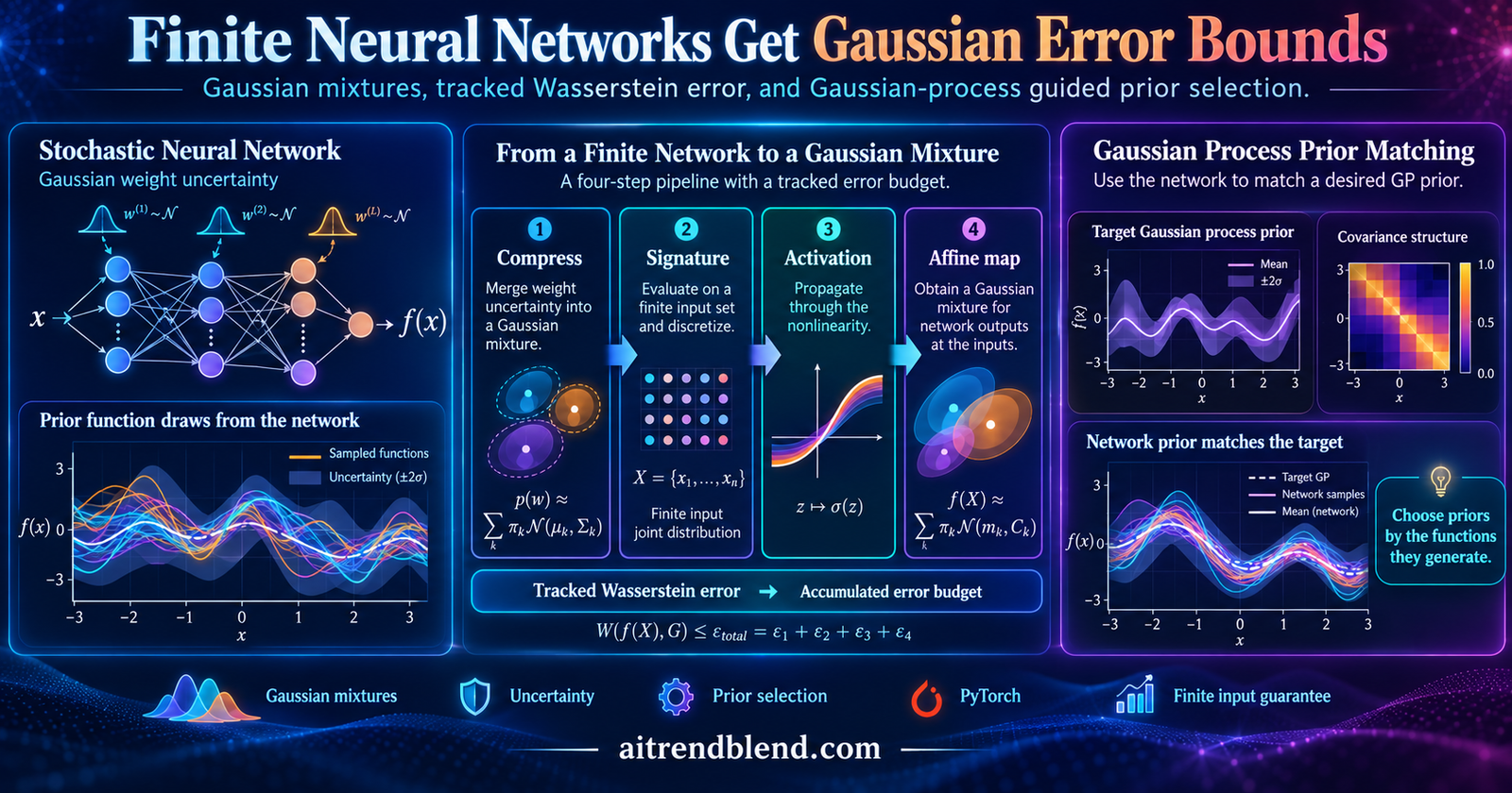
Before fitting a Bayesian regression network, a researcher draws functions from its prior. The intended behavior is smooth variation across the input range. The sampled curves instead look almost flat. The weight variances seemed reasonable. The functions they imply tell a different story.
That gap is the practical entry point to Finite Neural Networks as Mixtures of Gaussian Processes, published in the Journal of Machine Learning Research in January 2026. Steven Adams, Andrea Patanè, Morteza Lahijanian and Luca Laurenti develop a way to approximate the output distribution of a finite stochastic neural network with Gaussian mixtures, while tracking an upper bound on the approximation error.
The useful consequence runs in both directions. A Gaussian mixture can help explain a network’s uncertain predictions. A desired Gaussian process can also guide the choice of network priors. The paper provides an algorithmic framework and an experimental code repository, making prior selection a concrete workflow rather than a vague instruction to choose sensible weight scales.
- A finite stochastic network generally has a non Gaussian output distribution, even when its weights are Gaussian.
- The method approximates that distribution with a Gaussian mixture and accumulates Wasserstein error through the layers.
- The guarantee covers a finite set of inputs and their joint output distribution.
- Compression controls mixture size, while discrete signatures make nonlinear activation propagation tractable.
- Measured approximation errors can be small even when formal upper bounds are large.
- Matching a network’s function distribution to a Gaussian process gives a practical route to informative prior selection.
The infinite network result leaves a finite problem
A Gaussian process describes a distribution over functions through a mean and a covariance kernel. Evaluate a Gaussian process at finitely many inputs and the resulting output vector has a multivariate Gaussian distribution. The covariance tells you how predictions at different inputs move together, which is more informative than separate uncertainty bars.
The connection between neural networks and Gaussian processes is well established under suitable limiting assumptions. Lee and colleagues’ work on deep neural networks as Gaussian processes, cited by this paper, develops the equivalence for infinitely wide networks. The limit is a powerful analytical tool, but a trained network with a fixed architecture is a different object.
Nonlinear transformations of uncertain weights can produce skewed distributions, several modes or other departures from a single Gaussian. Training also changes the parameter distribution. Assuming independent and identically distributed parameters throughout a trained finite network is not generally justified by the infinite width analogy.
The authors therefore pose a more direct task. Given a finite stochastic network and a chosen set of inputs, construct a Gaussian mixture that is close to its joint output distribution. Report how close it is in the Wasserstein distance. A mixture retains more flexibility than a single Gaussian, and the error bound makes the approximation accountable.
Our Practical AI Tools hub collects workflows where these distinctions affect implementation. The related UQLM article concerns confidence scoring for language model answers. This paper addresses a different uncertainty problem, namely the distribution produced by random neural network parameters.
Which randomness does the model represent?
A stochastic neural network places a distribution over some of its parameters. Draw the parameters, evaluate the network and obtain a function realization. Draw again and the function may change. The distribution can represent a prior before observing labels or an approximate posterior after training.
Within a layer, the framework can accommodate parameter correlations and unequal distributions. That is part of what makes it more general than an independent weight limit. There is a boundary, however. The parameter distributions of different layers are assumed independent in the stated model. General correlations across layers are not automatically covered.
The main construction begins with Gaussian parameter distributions. Deterministic parameters can be treated as degenerate distributions. The paper also discusses extensions to other parameter distributions, including dropout, with extra approximation steps or specialized compression procedures. The extension should not be read as an identical cost or bound for every source of randomness.
This distinction also matters for the word posterior. Approximating a network trained with variational inference approximates the predictions associated with that variational weight distribution. It does not establish that the variational distribution itself equals the exact Bayesian posterior. There are two approximations, and their errors should not be merged into one reassuring number.
What the finite input guarantee says
Choose a finite collection of input points. Evaluate the same random network at all of them, sharing its parameter draw across the evaluations. The result is a joint output vector. Shared randomness creates correlations between the entries, and those correlations are part of the approximation target.
Equation 1. Problem 1 asks for a Gaussian mixture approximation within a specified error at the chosen finite input set.
The vector is not merely a list of unrelated marginal predictions. Two approximate models can have nearly identical uncertainty at each individual point but different relationships between those points. A joint approximation can detect that difference. This is particularly useful when the desired prior expresses smoothness across nearby inputs.
The finite set qualification is equally important. A guarantee at the selected points is not a uniform guarantee throughout an interval or image space. The authors identify approximation over compact input sets as a future direction. Selecting many points may be useful empirically, but it does not by itself turn the theorem into a continuum result.
“we focused on finding GMM approximations of neural networks at a finite set of input points”Adams and colleagues, Section 9, describing the scope of their guarantee
How the approximation moves through a layer
The first affine layer is the clean starting point. With a fixed input and Gaussian parameters, its output is Gaussian. The difficulty begins when that output passes through a nonlinear activation. A transformed Gaussian is generally not another Gaussian, so repeatedly carrying only a mean and covariance can lose the distribution’s shape.
The paper inserts a discrete approximation before the activation. Instead of applying the activation to every possible point of a continuous distribution, it places probability mass at a finite collection of locations. Each location can be transformed exactly. The next affine layer with Gaussian parameters then turns each transformed location into a Gaussian component.
That produces a mixture, whose component count can grow quickly. Before the next activation, the method compresses the mixture, builds a new discrete approximation and continues. Every compression and discretization contributes to the error budget. The nonlinear and affine maps determine how those errors propagate.
The order matters. Compressing an existing mixture is different from replacing the activated distribution with one convenient Gaussian. A valid implementation has to track which distribution each operation approximates and charge the error to that operation. The reported final distribution and bound are outputs of the same sequence.
The signature carries mass, not just sample points
The paper calls its discrete representation a signature. Locations partition the continuous support according to proximity. The probability assigned to a location is the probability mass in its region. This is not simply a set of equally weighted samples, and choosing attractive locations without calculating their masses changes the approximation.
Equation 2. For the nearest location partition, the signature error is the integrated squared transport cost, following Proposition 9.
For Gaussian components, the authors use grids aligned with covariance eigenvectors. In transformed coordinates, independent Gaussian directions make region probabilities and transport costs tractable. The grid is then transformed back. For a mixture, signatures are constructed component by component because different covariances can have different orientations.
Algorithm 2 allocates grid locations across directions using covariance information. A direction with more variation can need more locations. This is a practical reminder that discretization effort should follow the geometry of the distribution rather than treating every coordinate as equally demanding.
Compression preserves moments and records the cost
Algorithm 3 groups Gaussian components by clustering their means. Each cluster becomes a single Gaussian whose mean and covariance match the cluster mixture. The covariance includes the variation of the component means around the merged mean, not just the average of the individual covariances.
Equation 3. Moment matching for a cluster, as used in Algorithm 3.
Moment matching does not make the merged distribution identical to the original mixture. Distinct modes can disappear. The method therefore measures a mixture transport upper bound for the compression step. Increasing compression aggressively may reduce memory use while leaving an approximation that is harder to certify.
The paper uses a mixture Wasserstein quantity obtained from transporting component masses, with pairwise Gaussian transport costs. This is an upper bound on the ordinary Wasserstein distance between mixtures, not generally the exact distance. Keeping that distinction prevents a useful computational bound from being presented as an exact measurement.
Where the error budget comes from
Each layer inherits the error already accumulated and adds the cost of its current compression and signature. The activation and random affine map can amplify these discrepancies. Theorem 17 writes this propagation as a recurrence, with a multiplier based on the activation’s Lipschitz constant and an expected squared bound for the affine operator.
Equation 4. A schematic form of Theorem 17. Conservative valid bounds can replace the operator norm factor, while compression and signature terms must remain valid upper bounds.
Theorem 21 shows how appropriate mixture and grid sizes can achieve a chosen error tolerance on the finite input set. The construction can retain more components and use finer signatures when necessary. The promise is arbitrary precision under the assumptions, rather than arbitrary precision at a fixed small computing budget.
The cost can grow sharply. A grid with several locations along each uncertain direction requires the Cartesian product of those locations. More inputs, neurons and stochastic layers can enlarge that space. The theorem’s existence result should therefore be read alongside the practical need for compression and budget controls.
Another distinction concerns machine arithmetic. A mathematical upper bound is derived in exact terms. Numerical eigenvalue decompositions, transport solvers and rounded probabilities need care if software is supposed to issue a rigorous certificate. The editorial code below demonstrates the construction with ordinary floating point calculations and does not claim an outward rounded numerical proof.
The method tracks approximation error rather than assuming that a Gaussian surrogate is correct. A small measured discrepancy and a small proven upper bound are different achievements, and the experiments show that the gap can be large.
Measured errors and formal bounds tell different stories
Table 2 compares trained networks across regression and classification tasks. The authors use signatures of size 10 and compression size 5 in that table. Values are averaged over 100 randomly selected test points, and empirical discrepancies use 1,000 Monte Carlo samples from each distribution.
The metric is relative Wasserstein distance. Its denominator is the square root of the approximate distribution’s second moment. This makes the number a distributional comparison at a specified scale. It is not classification accuracy, an error rate or the proportion of predictions that are safe to trust.
| Dataset and architecture | Grid empirical | Grid formal upper bound | Cross empirical |
|---|---|---|---|
| NoisySines, one layer of 128 neurons, VI | 0.00130 | 0.13112 | 0.00041 |
| Kin8nm, one layer of 128 neurons, VI | 0.00012 | 0.04243 | 0.00012 |
| MNIST, one layer of 128 neurons, VI | 0.00058 | 0.05263 | 0.00037 |
| Fashion MNIST, two layers of 128 neurons, VI | 0.02787 | 1.45466 | 0.02228 |
| CIFAR-10, deterministic VGG 2 plus two layers of 128 neurons, VI | 0.04901 | 2.35686 | 0.02890 |
| MNIST, two layers of 64 neurons, dropout | 0.41874 | 1.37594 | 0.08603 |
VI means variational inference. The architecture descriptions follow the paper’s table notation. The empirical column is an estimate from sampled distributions, while the formal column is the method’s propagated upper bound. The fact that values are averaged across test points should not be mistaken for a certificate covering every possible input.
The cross shaped signature often has a smaller empirical error in the displayed examples. The authors explicitly state that their method cannot tractably provide formal bounds for that alternative. It is therefore not an automatic replacement when the objective is a formally bounded approximation. The table exposes a tradeoff between empirical efficiency and the available analysis.
The depth effect is also visible. A small empirical discrepancy can coexist with a formal bound above one for a deeper network. That bound does not certify a tight approximation, even if the sampled comparison looks favorable. It may reflect conservatism in propagation, an inadequate budget or both. The two columns answer different questions.
Dropout makes mixture flexibility more important
Table 3 varies compression size while holding the signature size at 100. For MNIST with one dropout layer of 64 neurons, the reported formal relative bound falls from 0.94371 at compression size 10 to 0.3571 at size 10,000. For two dropout layers of 64 neurons, the corresponding values are 1.37594 and 0.89742.
The same table is not uniformly monotone in every entry. In the stochastic VGG example, a bound rises slightly between two intermediate compression settings before falling at the largest one. It would be too strong to say that every increase in mixture size improves every reported bound. The broader evidence is that retaining more components can matter substantially for dropout distributions.
This supports a practical warning about replacing uncertain network outputs with a single Gaussian. Some tested variational networks are approximated adequately by that choice, while dropout models can need a richer mixture. The suitable number of components is a property of the distribution and the error budget, not a universal preference for simplicity.
Turning Gaussian process behavior into a network prior
The prior selection application reverses the approximation task. Begin with a Gaussian process whose kernel expresses the desired relationship between outputs. Then tune the distribution of the network’s weights so that its function distribution resembles the process on a selected set of inputs.
This approach makes an otherwise hidden choice visible. A weight prior can be easy to specify while implying undesirable functions. Looking at prior samples and their joint covariance reveals that mismatch before the network is trained on labels. The Gaussian process supplies a functional target rather than a list of arbitrary parameter variances.
Equation 5. Corollary 26 provides the unweighted sum bound. Equation 26 uses a weighted objective for tuning. The weighted objective is not generally itself the same upper bound.
The authors set the tuning coefficient to 0.01 in Section 8.3 and optimize centered Gaussian weight variances. The objective is piecewise differentiable, with care required around changes in clustering and degenerate covariance eigenvalues. This is a usable optimization idea, but differentiability does not remove numerical or nonconvex optimization difficulties.
| RBF length scale | Neurons per layer | Uninformative prior | Tran and colleagues | Proposed tuning |
|---|---|---|---|---|
| 1 | 64 | 0.97 | 0.30 | 0.25 |
| 1 | 128 | 0.46 | 0.30 | 0.25 |
| 0.75 | 64 | 1.09 | 0.39 | 0.32 |
| 0.75 | 128 | 0.56 | 0.39 | 0.31 |
| 0.5 | 64 | 1.23 | 0.53 | 0.47 |
| 0.5 | 128 | 0.69 | 0.53 | 0.43 |
These are empirical relative Wasserstein estimates evaluated at 20 test inputs, not predictive accuracy percentages. Proposed tuning has the lower discrepancy in all six displayed settings. The comparison supports the functional prior idea in the tested architectures and kernels, while leaving broader kernel families and larger problems for further evaluation.
The source contrasts its use of the second Wasserstein distance with the first Wasserstein distance in the earlier method. That should not be shortened into a claim that the first distance compares only means. Both are distances between distributions. The distinction concerns the transport cost, sensitivity to differences and the objectives actually optimized.
Does prior matching help after training?
The authors evaluate posterior predictions on Boston Housing, Concrete, Energy and Kin8nm. Figure 9 reports root mean square error and negative log likelihood across ten random test splits. Both metrics improve when the networks use the induced prior rather than the uninformative prior in the displayed comparison.
The Gaussian process still performs better in those results. The authors attribute the remaining difference to variational posterior approximation error. The fair interpretation is that functional prior selection helps the tested networks approach the target model’s behavior. It does not make a finite neural network identical to the Gaussian process after training.
The distinction between the two metrics matters. A lower root mean square error reflects better mean predictions. Negative log likelihood also considers the predictive distribution. Improvement in both is stronger evidence than improvement in a point prediction alone, but it is still evidence from selected regression datasets and inference procedures.
For a practitioner, the appropriate next step is to reproduce the prior samples, joint covariance and held out metrics on the intended task. Keep the training and evaluation choices consistent across the priors being compared. A desirable looking prior curve should start an experiment, not replace one.
Choose priors by inspecting the functions they imply. Then evaluate the trained predictive distribution separately. A useful functional prior and a well calibrated posterior are connected goals, but they are not the same guarantee.
Practical limits and a sensible adoption path
Start with a small input set and a modest stochastic architecture. Check whether the approximation budget produces a useful bound, then increase grid or mixture size deliberately. This is our implementation recommendation, drawn from the method’s structure. It is not a scaling result supplied by the paper.
Keep the joint dimension visible. A large set of inputs and many uncertain hidden features can make a tensor grid expensive even when each direction uses only a few locations. The paper supplies sophisticated allocation and alternative signatures, but the cost of accurate high dimensional approximation remains a real design constraint.
Check the source of randomness and the independence assumptions before reusing the framework. Gaussian variational weights, dropout masks and a fully correlated posterior across layers are different models. A bound derived for one should not be attached to another merely because their sampled predictions look similar.
Be cautious about the strength of the certificate. An upper bound far larger than the observed empirical discrepancy may be mathematically valid yet practically uninformative. Empirical closeness can justify further investigation, but it cannot tighten the theorem’s output without another argument or another budget.
The paper also includes a comparison of mean and covariance estimates on 30 inputs, using 10,000 Monte Carlo samples as a reference. The authors report a substantial speed advantage in that experiment. Treat the timing claim as tied to the studied configurations, rather than a universal guarantee that mixture propagation always beats sampling.
The open experimental repository linked from the paper is the appropriate starting point for reproducing its tables. The reference code in this article is a smaller educational implementation. It is useful for seeing the operations and their dependencies, with disclosed restrictions rather than an implied claim to reproduce the full experimental framework.
A more concrete way to reason about uncertain networks
The core achievement is a finite network approximation with a tracked distributional error. It extends the usefulness of Gaussian models beyond a limiting analogy while allowing a mixture to retain behavior that one Gaussian cannot express. The finite input set and stated parameter assumptions keep that achievement precise.
The conceptual change is to treat the Gaussian representation as an object whose approximation cost can be inspected. A mean and covariance are no longer the whole story. Signature error, compression error and amplification through layers become explicit parts of the explanation.
The approach is relevant wherever function behavior matters before labels are observed. Prior selection is the immediate application. Other uses may involve analyzing predictive correlations or constructing manageable surrogates for uncertain networks. The authors propose control and planning as future directions, rather than reporting a completed deployment in those settings.
The limitations remain visible. Joint dimensions can grow, formal bounds can be conservative and numerical differentiation needs care. The experiments show impressive small empirical errors alongside much larger bounds in several settings. Reporting both preserves the difference between an approximation that works in a test and one that has a tight guarantee.
Future work should improve bound tightness, computational scaling and guarantees beyond finite input collections. Practitioners can already benefit from a simpler habit supported by the paper. Inspect the functions your prior produces, decide what behavior you want and measure the mismatch before declaring the uncertainty meaningful.
A reasonable weight distribution is only a starting point. The functions it generates are the prior your model actually uses.
PyTorch reference implementation
The complete listing implements a small dense Gaussian case of the framework. It contains correlated Gaussian affine parameters within layers, shared parameter draws across inputs, Gaussian mixture compression, analytic signatures, propagated error estimates, finite input Gaussian process prior matching and a variational regression demonstration with evaluation and a smoke test.
It is editorial code, not the authors’ software. Fixed grids replace optimal grid allocation. A cluster assignment transport coupling gives a conservative compression estimate. The regression example uses ordinary diagonal Gaussian variational inference rather than the paper’s VOGN training. Convolutional networks, dropout specific compression and the authors’ stable eigenvalue derivatives are outside this listing.
The code uses ordinary floating point arithmetic and reports mathematical bound estimates rather than rigorously rounded numerical certificates. It passed a Python syntax check here. PyTorch was unavailable, so the included smoke test has not been executed here. Run it in an environment with PyTorch, NumPy and SciPy before extending the example.
"""Editorial dense-Gaussian special case of Adams et al., JMLR 27(33), 2026.
Python 3.10+, PyTorch, NumPy and SciPy are required.
Complete tiny workflow: stochastic NN, GMM compression, analytic signatures,
layer error propagation, GP-prior matching, regression VI, evaluation, smoke test.
Not the authors' code. Not a reproduction of VGG, dropout or paper tables.
Fixed per-eigendimension grids replace optimal allocation in Algorithm 2.
Ordinary floating point computations are NOT outward-rounded certified arithmetic.
Degenerate eigenvalues may make autograd unstable; the paper uses a special
stable derivative implementation that is not reproduced here.
"""
from dataclasses import dataclass
from functools import lru_cache
from itertools import product
import math
import numpy as np
from scipy.optimize import linprog
from scipy.special import ndtr
import torch
from torch import nn
from torch.nn import functional as F


@dataclass
class Mixture:
    mass: torch.Tensor  # [components]
    mean: torch.Tensor  # [components, dimension]
    cov: torch.Tensor   # [components, dimension, dimension]

    def moments(self):
        mean = (self.mass[:, None] * self.mean).sum(0)
        centered = self.mean - mean
        covariance = (self.mass[:, None, None] *
                      (self.cov + centered[:, :, None] * centered[:, None, :])).sum(0)
        return mean, covariance

    def second_moment(self):
        return (self.mass * (self.mean.square().sum(-1) +
                            self.cov.diagonal(dim1=-2, dim2=-1).sum(-1))).sum()

    @torch.no_grad()
    def sample(self, count):
        ix = torch.multinomial(self.mass, count, replacement=True)
        vals, vecs = torch.linalg.eigh(self.cov[ix])
        factor = vecs * vals.clamp_min(0).sqrt().unsqueeze(-2)
        noise = torch.randn(count, self.mean.size(1), dtype=self.mean.dtype)
        return self.mean[ix] + torch.einsum('bij,bj->bi', factor, noise)


def psd_sqrt(matrix):
    """No jitter: clipping roundoff is a numerical step, not exact certification."""
    matrix = (matrix + matrix.T) / 2
    vals, vecs = torch.linalg.eigh(matrix)
    return (vecs * vals.clamp_min(0).sqrt().unsqueeze(0)) @ vecs.T


def gaussian_w2_squared(m1, c1, m2, c2):
    root = psd_sqrt(c1)
    middle = psd_sqrt(root @ c2 @ root)
    return ((m1 - m2).square().sum() + torch.trace(c1 + c2 - 2 * middle)).clamp_min(0)


def mixture_w2_upper(a, b):
    """MW2 via the finite transport LP, Definition 2. This upper bounds W2.
    The solved plan is held fixed for local differentiation of the optimal value.
    Solver tolerances and PSD roundoff prevent a rigorous machine certificate.
    """
    rows, cols = len(a.mass), len(b.mass)
    if rows * cols > 20000:
        raise ValueError('This small reference implementation limits the transport LP.')
    cost = torch.stack([torch.stack([
        gaussian_w2_squared(a.mean[i], a.cov[i], b.mean[j], b.cov[j])
        for j in range(cols)]) for i in range(rows)])
    constraints = np.zeros((rows + cols, rows * cols))
    for i in range(rows): constraints[i, i * cols:(i + 1) * cols] = 1
    for j in range(cols): constraints[rows + j, j::cols] = 1
    rhs = np.r_[a.mass.detach().numpy(), b.mass.detach().numpy()]
    solution = linprog(cost.detach().numpy().ravel(), A_eq=constraints,
                       b_eq=rhs, bounds=(0, None), method='highs')
    if not solution.success:
        raise RuntimeError('Mixture transport LP failed: ' + solution.message)
    plan = torch.as_tensor(solution.x.reshape(rows, cols), dtype=cost.dtype)
    # Plan derivatives in the marginals are not included. For prior tuning below,
    # target is one Gaussian; the unique plan is a.mass and is differentiable.
    if cols == 1:
        plan = a.mass[:, None]
    return (plan * cost).sum().clamp_min(0).sqrt()


def compress(q, maximum, iterations=20):
    """Algorithm 3: Lloyd clustering of means, then moment matching.
    A valid cluster-assignment coupling yields a conservative compression bound.
    This avoids an additional LP while remaining an upper bound in exact math.
    """
    if maximum < 1:
        raise ValueError('Compression size must be positive.')
    count = len(q.mass)
    if count <= maximum:
        return q, q.mean.new_zeros(())
    with torch.no_grad():
        detached = q.mean.detach()
        centers = detached[torch.linspace(0, count - 1, maximum).long()].clone()
        for _ in range(iterations):
            labels = torch.cdist(detached, centers).argmin(1)
            for j in range(maximum):
                if (labels == j).any(): centers[j] = detached[labels == j].mean(0)
        labels = torch.cdist(detached, centers).argmin(1)
    masses, means, covs = [], [], []
    compression_cost = q.mean.new_zeros(())
    for j in range(maximum):
        ix = torch.where(labels == j)[0]
        if not len(ix): continue
        mass = q.mass[ix].sum()
        normalized = q.mass[ix] / mass
        mean = (normalized[:, None] * q.mean[ix]).sum(0)
        delta = q.mean[ix] - mean
        cov = (normalized[:, None, None] *
               (q.cov[ix] + delta[:, :, None] * delta[:, None, :])).sum(0)
        for i in ix:
            compression_cost = compression_cost + q.mass[i] * gaussian_w2_squared(
                q.mean[i], q.cov[i], mean, cov)
        masses.append(mass); means.append(mean); covs.append(cov)
    result = Mixture(torch.stack(masses), torch.stack(means), torch.stack(covs))
    return result, compression_cost.clamp_min(0).sqrt()


@lru_cache(maxsize=32)
def normal_grid(nodes):
    """Lloyd fixed-point quantizer for N(0,1), including infinite tails.
    Returns locations, cell masses and integrated squared transport error.
    """
    if nodes < 1: raise ValueError('At least one grid node is required.')
    centers = np.linspace(-2, 2, nodes) if nodes > 1 else np.array([0.])
    phi = lambda x: np.exp(-0.5 * x * x) / math.sqrt(2 * math.pi)
    for _ in range(100):
        cuts = np.r_[-np.inf, (centers[:-1] + centers[1:]) / 2, np.inf]
        mass = ndtr(cuts[1:]) - ndtr(cuts[:-1])
        first = phi(cuts[:-1]) - phi(cuts[1:])
        updated = first / np.maximum(mass, 1e-300)
        if np.max(np.abs(updated - centers)) < 1e-12:
            centers = updated
            break
        centers = updated
    cuts = np.r_[-np.inf, (centers[:-1] + centers[1:]) / 2, np.inf]
    mass = ndtr(cuts[1:]) - ndtr(cuts[:-1])
    first = phi(cuts[:-1]) - phi(cuts[1:])
    # Limit x*phi(x) is zero at either infinity.
    finite = np.isfinite(cuts)
    xphi = np.zeros_like(cuts)
    xphi[finite] = cuts[finite] * phi(cuts[finite])
    second = mass + xphi[:-1] - xphi[1:]
    error = np.sum(second - 2 * centers * first + centers ** 2 * mass)
    return centers, mass, max(float(error), 0.)


def signature(q, nodes=3, max_particles=4096):
    """Algorithm 2 structure, with fixed grids rather than optimal allocation.
    Keeps every strictly positive eigenvalue; dropping one would change the model.
    Singular directions use a deterministic zero in standardized coordinates.
    """
    centers_np, mass_np, scalar_error = normal_grid(nodes)
    centers = torch.as_tensor(centers_np, dtype=q.mean.dtype)
    mass = torch.as_tensor(mass_np, dtype=q.mean.dtype)
    locations, masses = [], []
    error2 = q.mean.new_zeros(())
    for i in range(len(q.mass)):
        covariance = (q.cov[i] + q.cov[i].T) / 2
        values, vectors = torch.linalg.eigh(covariance)
        tolerance = 1e-10 * max(float(covariance.detach().abs().max()), 1.)
        if float(values.detach().min()) < -tolerance:
            raise RuntimeError('Covariance is not numerically positive semidefinite.')
        values = values.clamp_min(0)
        active = torch.where(values.detach() > 0)[0]
        count = nodes ** len(active)
        if len(locations) + count > max_particles:
            raise ValueError('Signature grid exceeds budget; reduce dimension or grid size.')
        choices = list(product(range(nodes), repeat=len(active)))
        if not len(active): choices = [()]
        for choice in choices:
            point = q.mean[i]
            probability = q.mass[i]
            for d, node in zip(active, choice):
                point = point + vectors[:, d] * values[d].sqrt() * centers[node]
                probability = probability * mass[node]
            locations.append(point); masses.append(probability)
        error2 = error2 + q.mass[i] * values.sum() * scalar_error
    return torch.stack(locations), torch.stack(masses), error2.clamp_min(0).sqrt()


class GaussianAffine(nn.Module):
    """Dense affine parameters are jointly Gaussian within each layer.
    Same sampled weights are shared across all evaluated input points.
    Layers have independent parameter distributions, as required by the model.
    """
    def __init__(self, inp, out, initial_std=0.15):
        super().__init__()
        self.inp, self.out = inp, out
        size = out * (inp + 1)
        self.mean = nn.Parameter(torch.randn(size, dtype=torch.float64) * 0.2)
        chol = torch.zeros(size, size, dtype=torch.float64)
        chol.diagonal().fill_(math.log(math.expm1(initial_std)))
        self.raw_chol = nn.Parameter(chol)

    def covariance(self):
        factor = torch.tril(self.raw_chol, -1) + torch.diag(F.softplus(self.raw_chol.diagonal()))
        return factor @ factor.T

    def weight_lipschitz_bound(self):
        index = torch.arange(self.out * (self.inp + 1)).reshape(self.out, self.inp + 1)[:, :-1].flatten()
        # sqrt E||W||_F^2 is >= sqrt E||W||_2^2.
        return (self.mean[index].square().sum() + self.covariance().diagonal()[index].sum()).sqrt()

    def design(self, values):
        # values: [components, evaluation points, input features]
        count, npoints, _ = values.shape
        augmented = torch.cat((values, values.new_ones(count, npoints, 1)), -1)
        identity = torch.eye(self.out, dtype=values.dtype)
        blocks = torch.einsum('oj,bnf->bnjof', identity, augmented)
        return blocks.reshape(count, npoints * self.out, self.out * (self.inp + 1))

    def push(self, values, mass):
        design = self.design(values)
        mean = design @ self.mean
        cov = design @ self.covariance() @ design.transpose(-1, -2)
        return Mixture(mass, mean, cov)

    def draw(self, samples):
        factor = torch.linalg.cholesky(self.covariance())
        return self.mean + torch.randn(samples, len(self.mean), dtype=self.mean.dtype) @ factor.T


class FiniteGaussianNetwork(nn.Module):
    def __init__(self, widths=(1, 1, 1), activation='tanh'):
        super().__init__()
        if len(widths) < 2 or activation not in ('tanh', 'relu'):
            raise ValueError('Use positive widths and a supported Lipschitz activation.')
        self.layers = nn.ModuleList([GaussianAffine(a, b) for a, b in zip(widths[:-1], widths[1:])])
        self.activation = torch.tanh if activation == 'tanh' else F.relu

    def approximate(self, x, nodes=3, components=2):
        """Algorithm 1. Returns the JOINT distribution on finite input set x."""
        x = x.to(dtype=torch.float64, device='cpu')
        q = self.layers[0].push(x.unsqueeze(0), x.new_ones(1))
        error = x.new_zeros(())
        npoints = len(x)
        for layer in self.layers[1:]:
            compressed, compression = compress(q, components)
            particles, mass, quantization = signature(compressed, nodes)
            values = self.activation(particles.reshape(len(particles), npoints, layer.inp))
            q = layer.push(values, mass)
            error = layer.weight_lipschitz_bound() * (error + compression + quantization)
        return q, error

    def sample_functions(self, x, samples):
        values = x.unsqueeze(0).expand(samples, *x.shape)
        for i, layer in enumerate(self.layers):
            if i: values = self.activation(values)
            parameters = layer.draw(samples).reshape(samples, layer.out, layer.inp + 1)
            values = torch.einsum('sni,soi->sno', values, parameters[:, :, :-1]) + parameters[:, None, :, -1]
        return values.reshape(samples, -1)


def gp_target(x, lengthscale=0.5, variance=1.):
    """Scalar zero-mean RBF GP evaluated jointly at finite x."""
    covariance = variance * torch.exp(-torch.cdist(x, x).square() / (2 * lengthscale ** 2))
    return Mixture(x.new_ones(1), x.new_zeros(1, len(x)), covariance.unsqueeze(0))


def prior_loss(network, x, target, beta=0.01, nodes=3, components=2):
    if not 0 <= beta <= 1: raise ValueError('beta must lie in [0,1].')
    q, approximation = network.approximate(x, nodes, components)
    mismatch = mixture_w2_upper(q, target)
    # Eq. 26 is a weighted tuning objective. The certificate is the UNWEIGHTED sum.
    return beta * approximation + (1 - beta) * mismatch, approximation + mismatch


def tune_prior(network, x, target, steps=10, lr=1e-3):
    """Train prior parameters only; no response labels enter this objective.
    Tiny finite grid. Extend stable eigen derivatives before using larger grids.
    """
    optimizer = torch.optim.Adam(network.parameters(), lr=lr)
    history = []
    for _ in range(steps):
        optimizer.zero_grad(set_to_none=True)
        loss, bound = prior_loss(network, x, target)
        loss.backward()
        for parameter in network.parameters():
            if parameter.grad is not None and not torch.isfinite(parameter.grad).all():
                raise RuntimeError('Nonfinite gradient; inspect covariance degeneracy.')
        optimizer.step()
        history.append((float(loss.detach()), float(bound.detach())))
    return history


class VariationalRegressor(nn.Module):
    """Editorial diagonal-Gaussian VI, NOT VOGN used in the paper's experiments."""
    def __init__(self, prior):
        super().__init__()
        self.prior = prior
        for parameter in self.prior.parameters(): parameter.requires_grad_(False)
        self.mean = nn.ParameterList([nn.Parameter(layer.mean.detach().clone()) for layer in prior.layers])
        self.logstd = nn.ParameterList([nn.Parameter(torch.full_like(m, -3.)) for m in self.mean])

    def sample_predictions(self, x, count):
        values = x.unsqueeze(0).expand(count, *x.shape)
        for i, (layer, mean, logstd) in enumerate(zip(self.prior.layers, self.mean, self.logstd)):
            if i: values = self.prior.activation(values)
            parameter = mean + logstd.exp() * torch.randn(count, len(mean), dtype=x.dtype)
            parameter = parameter.reshape(count, layer.out, layer.inp + 1)
            values = torch.einsum('sni,soi->sno', values, parameter[:, :, :-1]) + parameter[:, None, :, -1]
        return values.squeeze(-1)

    def kl(self):
        total = self.mean[0].new_zeros(())
        for layer, mean, logstd in zip(self.prior.layers, self.mean, self.logstd):
            covariance = layer.covariance().detach()
            inverse = torch.linalg.inv(covariance)
            delta = mean - layer.mean.detach()
            logdet = torch.linalg.slogdet(covariance)[1]
            total = total + 0.5 * (torch.dot(inverse.diagonal(), (2 * logstd).exp()) +
                    delta @ inverse @ delta - len(mean) + logdet - 2 * logstd.sum())
        return total

    def loss(self, x, y, noise=0.1, samples=8):
        predictions = self.sample_predictions(x, samples)
        nll = (0.5 * ((predictions - y) / noise).square() + math.log(noise) +
               0.5 * math.log(2 * math.pi)).sum(-1).mean()
        return nll + self.kl()


def train_regression(model, x, y, steps=20, lr=1e-3):
    optimizer = torch.optim.Adam([p for p in model.parameters() if p.requires_grad], lr=lr)
    for _ in range(steps):
        optimizer.zero_grad(set_to_none=True)
        loss = model.loss(x, y)
        if not torch.isfinite(loss): raise RuntimeError('Nonfinite VI loss.')
        loss.backward(); optimizer.step()
    return model


@torch.no_grad()
def evaluate(model, x, y, samples=100, noise=0.1):
    predictions = model.sample_predictions(x, samples)
    mean = predictions.mean(0)
    component_logp = -0.5 * ((predictions - y) / noise).square() - math.log(noise) - 0.5 * math.log(2 * math.pi)
    predictive_logp = torch.logsumexp(component_logp, 0) - math.log(samples)
    return {'rmse': float((mean - y).square().mean().sqrt()),
            'nll': float(-predictive_logp.mean())}


def smoke_test():
    """Dummy data check. No research accuracy or rigorous certificate is claimed."""
    torch.manual_seed(7)
    torch.set_num_threads(1)
    x = torch.tensor([[-0.4], [0.6]], dtype=torch.float64)
    network = FiniteGaussianNetwork()
    q, bound = network.approximate(x, nodes=3, components=2)
    assert q.mean.shape[1] == len(x)
    assert torch.allclose(q.mass.sum(), torch.tensor(1., dtype=x.dtype), atol=1e-8)
    assert torch.isfinite(bound) and bound >= 0
    assert torch.isfinite(q.sample(20)).all()
    assert torch.isfinite(network.sample_functions(x, 20)).all()
    # A two-point target illustrates joint GP structure. One point is used for
    # gradient smoke training to avoid degenerate covariance derivatives.
    joint_target = gp_target(x)
    assert torch.isfinite(mixture_w2_upper(q, joint_target))
    train_x = x[:1]
    tune_prior(network, train_x, gp_target(train_x), steps=2)
    regression = VariationalRegressor(network)
    data_x = torch.linspace(-1, 1, 12, dtype=x.dtype)[:, None]
    y = torch.sin(2 * data_x[:, 0]) + 0.05 * torch.randn(12, dtype=x.dtype)
    train_regression(regression, data_x, y, steps=2)
    print(evaluate(regression, data_x, y, samples=20))
    print('Mechanics checked on dummy data, not paper benchmark reproduction.')


if __name__ == '__main__':
    smoke_test()
Frequently asked questions
Is a finite neural network exactly a Gaussian process?
Generally no. A finite network with random Gaussian weights and nonlinear activations can have non Gaussian output distributions. The paper constructs Gaussian mixture approximations with tracked error.
Does the error bound cover every possible input?
No. The stated guarantee concerns a chosen finite input set and its joint output distribution. A uniform guarantee over a continuous input domain requires further work.
Do the cross signatures have the same formal bound?
No. The paper evaluates their empirical approximation quality, but reports that formal error computation for those signatures is intractable with the stated approach.
Does a small approximation bound prove prediction accuracy?
No. It concerns closeness between output distributions under the stated model. Predictive accuracy, posterior calibration and the quality of a variational weight distribution require separate evaluation.
How does Gaussian process matching choose a network prior?
It tunes the weight distribution so the network produces a function distribution close to a desired Gaussian process at selected inputs. The trained posterior still depends on data and the inference method.
Does the included code reproduce the authors’ experiments?
No. It is an educational dense Gaussian implementation with disclosed simplifications. Python syntax was checked, but its PyTorch smoke test was not executed here.
Inspect the source and the experimental implementation
The paper includes the proofs, algorithm details, additional signatures and the complete experimental comparisons.
Read the JMLR paperAuthors’ experimental codeAdams, S., Patanè, A., Lahijanian, M., and Laurenti, L. (2026). Finite Neural Networks as Mixtures of Gaussian Processes, From Provable Error Bounds to Prior Selection. Journal of Machine Learning Research, 27(33), pages 1 to 52. Title punctuation simplified. Official publication record.
This analysis is based on the published paper and an independent evaluation of its claims.