
Key points
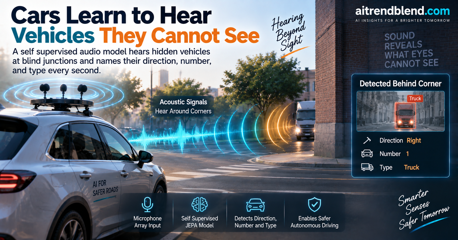
- The work builds an onboard acoustic perception system for driverless cars that detects vehicles hidden beyond line of sight, using only the raw audio from an eight microphone roof array.
- It is the first such system to answer three questions at once every second, the direction of a hidden vehicle, how many vehicles are present, and their type, without separating the overlapping sounds first.
- A self supervised stage inspired by the Joint Embedding Predictive Architecture teaches the encoder to predict a future sound from a past one, which turns out to learn a stronger representation than plain supervised training.
- On the authors’ T junction data the model reaches 81.8 percent direction accuracy, 94.5 percent counting accuracy, and 93.7 percent vehicle type accuracy, beating every prior method they compare against.
- The honest catch is transfer. Dropped cold onto a moving overtaking scenario it never heard, accuracy collapses, and it needs a handful of labeled examples to recover.
Why the eyes of a car go blind at a blind corner
Think about what safe driving actually requires. Not just reacting to what is in front of you, but anticipating what is about to be. A pedestrian stepping from behind a parked truck, a scooter darting out of a side street, a bus swinging wide around a corner. The dangerous agents are often the ones you cannot see yet, and every camera and lidar on a modern autonomous vehicle shares one hard limit. They need a clear line of sight. Point them at a wall and they see a wall.
Radar does a little better, since it can pass through plastic bumpers and glass, but it still cannot see through the solid metal of a vehicle sitting between the sensor and the thing you care about. So at the exact geometry that causes the worst intersection accidents, the blind junction where two streets meet behind buildings, the whole visual sensor suite goes quiet at the same moment.
Sound does not play by those rules. Acoustic waves bend and wrap around obstacles, they arrive from every direction at once, and they carry information about what made them long before the source becomes visible. Earlier research already showed that a microphone array can flag an approaching car around a corner before it appears. The problem was that those systems answered only one narrow question. Either which direction the sound came from, or what kind of vehicle it was, and only ever for a single vehicle at a time. Real streets do not cooperate like that.
The core idea, hearing more than one thing you cannot see
This is where the new work pushes forward. The authors, Katerina Vinciguerra and Letizia Marchegiani at the University of Parma with Moritz Brandes and Danilo Hollosi at the Fraunhofer institute in Oldenburg, built a single system that answers three questions simultaneously, once per second, from raw microphone audio alone. Which direction is a hidden vehicle arriving from. How many vehicles are out there. And what type each one is, a car or a van or one of each.
The clever move is what they refused to do. The obvious way to handle two overlapping engine sounds is to separate them first, split the mixed audio into individual sources, then analyze each. Except sound source separation in the messy real world remains a genuinely unsolved problem. So they skipped it entirely. The model learns to read the combined acoustic signature of a scene directly, treating the overlap of a car and a van as its own pattern to recognize rather than a mixture to untangle. That keeps the whole thing lightweight enough to run onboard and honest about its own scope. The authors call it a proof of concept for up to two simultaneous vehicles, and they say so plainly.
What changed from earlier acoustic work
Two threads of prior research meet here. On one side, acoustic vehicle detection around corners, which had been stuck at single vehicle direction estimation. On the other, the roadside traffic monitoring systems from the audio research community, which can count and classify vehicles but sit on fixed poles and report once a minute, far too slow and too stationary to help a car decide what to do in the next moment. This paper takes the onboard, one second, multiple vehicle setting that neither camp had covered and treats all three tasks as one joint problem.
Teaching an encoder to listen without any labels
The heart of the method is how the audio encoder is trained, and it borrows a fashionable idea from self supervised learning called the Joint Embedding Predictive Architecture, usually shortened to JEPA. The intuition is worth slowing down on, because it is doing the real work.
Most self supervised audio models learn by reconstruction. Mask part of a sound, then try to rebuild the missing waveform sample by sample. The trouble is that a lot of a raw waveform is perceptually irrelevant detail, and forcing a model to reproduce it wastes capacity on noise. JEPA changes the target. Instead of rebuilding the raw signal, it predicts the abstract latent representation of a missing region from the surrounding context. You are no longer asked to redraw the sound. You are asked to anticipate what the sound will mean.
Two encoders and a guessing game
Concretely the system keeps two copies of the encoder. An online encoder that learns by gradient descent, and a target encoder whose weights are a slow moving average of the online one. A small predictor network looks at the latent produced from a past one second of audio and tries to guess the latent that the target encoder will produce for a future one second of audio. The prediction error is the entire training signal, and no human label is involved anywhere.
The target encoder never receives a gradient. It only drifts toward the online encoder through an exponential moving average, a trick borrowed from the well known self supervised method BYOL that stops the whole thing from collapsing into a trivial constant answer without needing negative examples to push against.
Why it deliberately skips the middle second
Here is a detail that reveals real care. Given three consecutive one second frames, the model predicts the third from the first and throws the middle one away during pretraining. Why leave out the obvious in between frame? Because predicting the very next instant is too easy. A model can cheat by just extending the immediate spectral content forward, which teaches it almost nothing. Forcing a two second jump makes the encoder capture longer range acoustic dynamics, the way an engine note swells and shifts as a vehicle actually moves. The ablation table confirms it. The two step horizon reaches 81.8 percent direction accuracy against 80.8 for the one step version, and 79.3 for a variant that fills in the middle from both sides, which drifts back toward reconstruction and loses the forecasting benefit.
From a latent sound to three answers at once
Once the encoder is trained, the predictor is thrown away and the encoder is reused. Its architecture is deliberately small. Three strided one dimensional convolution blocks with a kernel size of nine walk across the raw waveform, widening from sixty four to one hundred twenty eight to two hundred fifty six channels, then a global average pool over time and a linear layer produce a two hundred fifty six dimensional summary of one second of eight channel audio.
For the actual task, three consecutive seconds are each encoded into a latent, and a bidirectional recurrent network reads the short sequence forward and backward to aggregate how the scene evolves. Its final state passes through a shared block with heavy dropout, then splits into three small classification heads. One predicts direction across five labels, left, front, right, none, and both sides at once. One predicts the count as zero, one, or two vehicles. One predicts type as car, van, one of each, or none. All three train together under a single combined loss that weights the harder direction task five times more heavily than the others.
Fine tuning happens in two gentle phases. For the first five epochs the encoder stays frozen while only the recurrent aggregator and the heads learn. Then the encoder unfreezes and joins in, but at a learning rate one hundred times smaller, so the self supervised representation adapts to the labels without forgetting what it learned. It is a careful recipe, and the care shows up in the results.
The model never separates the sounds. It learns to read the combined acoustic fingerprint of a whole scene, and that refusal to untangle is what keeps it small enough to run onboard.A plain reading of the method
The dataset they had to build from scratch
No public dataset existed for this problem, so the team collected their own. They mounted three cameras and a GPS unit on a vehicle roof directly above an octagonal array of eight microphones sampling at forty eight kilohertz, then recorded at a solar park in Oldenburg, Germany. To keep the model from simply memorizing one engine, they used two different cars and two different vans across the trials.
The recordings split into two very different settings. In the T junction set the host vehicle sits still while one or two vehicles approach from hidden side streets, giving 6,827 labeled one second frames. In the take over set the host vehicle is itself moving while others overtake it, a much smaller 3,005 frames. Crucially the take over set is held out from everything, including the self supervised pretraining, so it functions as a genuinely unseen world for testing transfer. Labels came from running a modern object detector on the camera footage and correcting its mistakes by hand.
What the numbers actually show
On the stationary T junction data the system is strong across all three tasks at once. The fully fine tuned model reaches 81.8 percent on direction, 94.5 percent on counting, and 93.7 percent on vehicle type. The comparison that matters most is against the only prior method that also does all three tasks, a baseline from the audio traffic monitoring community, which the new model beats by a wide margin on direction and type and a smaller one on counting.
| Method or configuration | Direction (%) | Count (%) | Type (%) |
|---|---|---|---|
| Recurrent baseline, no pretraining | 33.7 | 47.0 | 40.0 |
| Roadside monitoring baseline | 67.5 | 89.5 | 66.9 |
| Array processing with a linear classifier | 53.4 | – | – |
| Direction network with convolutions | 61.9 | – | – |
| Spectrogram with convolutions | 75.0 | – | – |
| Self supervised encoder, frozen | 79.9 | 94.1 | 93.2 |
| Self supervised encoder, fine tuned (ours) | 81.8 | 94.5 | 93.7 |
Two things in that table deserve a pause. First, the recurrent baseline with no self supervised pretraining lands at a dismal 33.7 percent on direction, which tells you the pretraining is not a nice extra but the load bearing wall of the whole design. Second, the frozen encoder is almost as good as the fine tuned one. The representation learned with zero labels is already doing nearly all the work, and letting the labels nudge it further buys only a couple of points. That is a strong signal that the self supervised task genuinely captured something about how vehicles sound as they move.
The per class breakdown adds texture. Counting recall stays above ninety three percent for every class, which is remarkable given that nothing in the architecture was designed for counting. The model simply learned that one engine and two engines leave different fingerprints. Vans are the easiest vehicle to name, at ninety seven percent recall, thanks to their distinctive low frequency rumble. The hardest label is the front direction at sixty percent, and the authors trace the errors to the moments when a vehicle transitions from the side into the frontal cone, where the boundary between labels is genuinely fuzzy rather than acoustically meaningful.
The honest part, a road it has never heard
None of this comes for free, and the paper is refreshingly candid about where the approach struggles. The real test of a driving system is not the data it trained on but a situation it has never met, and the held out take over set is exactly that. The host vehicle is now moving, the wind and road noise are different, and there is a whole new direction label, a vehicle approaching from behind, that never appeared in training.
Dropped in cold with zero examples, the model falls apart. Direction accuracy is 2.3 percent, which is effectively zero by construction since the new rear label has never received a single gradient. Counting and type collapse to single digits too. This is the distribution shift problem in its rawest form, and it is worth stating bluntly because a reader skimming only the headline accuracy would never guess it.
The recovery is where the self supervised foundation pays off. With just five labeled examples from the new scenario, direction accuracy jumps to around fifty five percent, and with ten it reaches roughly seventy percent. The team tried three different adaptation strategies, from retraining only the heads to re running the self supervised stage on the new audio, and found they were all essentially equivalent. The frozen representation already carried enough structure that a light touch of new labels was all it took. That equivalence is quietly important. It means the expensive option, re pretraining on the new environment, is not worth the trouble, and a few labeled clips will do.
A head start measured in seconds
The most compelling number in the paper is not an accuracy at all. It is a measure of how much warning the system buys. For each scenario where a vehicle enters the field of view from the side, the authors measured the longest unbroken run of correct predictions ending just before the vehicle became visible to the camera. The mean was 4.6 seconds, with a median of 5.0. In more than three quarters of scenarios the model gave at least one second of advance notice, and in nearly two thirds it gave at least three.
Three to five seconds does not sound like much until you translate it into a planner’s world. At urban speeds that is the difference between easing off the accelerator early and slamming the brakes late. It is time to plan a gentle response instead of an emergency one. For anyone building anticipatory perception, that head start is the entire point, and it is the same instinct behind work that pushes forecasting earlier in the pipeline, such as our look at how MC-DeTra sharpens driving forecasts at no inference cost. It also sits naturally alongside sensor fusion research that fights the same blindness from the visual side, like multi modal perception for autonomous racing and detectors that stay reliable when a sensor fails. Readers curious about the label free training idea at the center of this method will find a useful companion in our explainer on self supervised video understanding without human labels.
Where it still struggles
The limitations are real and the authors name most of them. The system handles at most two simultaneous vehicles, and busy traffic will demand more. The front direction stays the weakest class because the label boundaries are drawn by camera cones rather than by anything the sound itself respects. Under the class imbalance of the moving scenario, some directions stay stubbornly hard, with the right side barely recognized and the left side behaving erratically as more examples are added, a sign that the model has not yet built a stable spatial map.
There is also a quieter caveat worth flagging. The whole evaluation rests on one dataset collected by one team at one location with a specific microphone geometry. The transfer experiment shows the model is sensitive to changes in scenario, which means a different vehicle, a different array, or a different acoustic environment could shift the numbers. The paper is a careful proof of concept, and it reads as one, not as a deployable product. The proposed path forward is to move from discrete direction labels toward continuous angle regression and to fold the audio into a full multi sensor system, which is the sensible next step.
The full method, in runnable PyTorch
The block below is a faithful, self contained reference implementation of the two stage pipeline, including the convolutional waveform encoder, the JEPA style predictor and moving average target, the self supervised loss, the bidirectional aggregator with three heads, both training loops, and a smoke test on dummy multichannel audio. It follows the architecture described in the paper. Read it as a teaching implementation you can run and extend rather than the authors’ exact code, which was not released publicly.
# Predictive audio representations for beyond line of sight vehicle detection.
# Stage 1 JEPA-style self-supervised pretraining on raw 8-channel waveforms,
# Stage 2 supervised BiLSTM with three heads (direction, count, type).
import copy
import torch
import torch.nn as nn
import torch.nn.functional as F

M_MICS = 8; FS = 48000; D = 256          # channels, sample rate, latent dim

# ----------------------------------------------------------------------
# 1. Waveform encoder: 3 strided 1D conv blocks -> GAP -> linear (D)
# ----------------------------------------------------------------------
class WaveEncoder(nn.Module):
    def __init__(self, in_ch=M_MICS, d=D):
        super().__init__()
        chans = [in_ch, 64, 128, 256]
        blocks = []
        for i in range(3):
            blocks += [nn.Conv1d(chans[i], chans[i + 1], kernel_size=9,
                                 stride=2, padding=4, bias=False),
                       nn.BatchNorm1d(chans[i + 1]), nn.ReLU(inplace=True)]
        self.conv = nn.Sequential(*blocks)
        self.fc = nn.Linear(256, d)                    # projection after pooling

    def forward(self, x):
        # x: (B, 8, L) one second of raw multichannel audio
        h = self.conv(x)                            # (B, 256, L')
        h = h.mean(dim=-1)                          # global average pool over time
        return self.fc(h)                            # (B, D)

class Predictor(nn.Module):
    """Two-layer MLP that forecasts a future latent from a past one."""
    def __init__(self, d=D):
        super().__init__()
        self.net = nn.Sequential(nn.Linear(d, d), nn.ReLU(inplace=True), nn.Linear(d, d))
    def forward(self, z): return self.net(z)

# ----------------------------------------------------------------------
# 2. Stage 1: JEPA-style self-supervised pretraining
# ----------------------------------------------------------------------
class JEPAPretrainer(nn.Module):
    def __init__(self, m=0.99):
        super().__init__()
        self.online = WaveEncoder()
        self.target = copy.deepcopy(self.online)     # EMA target, no gradient
        for p in self.target.parameters(): p.requires_grad_(False)
        self.predictor = Predictor()
        self.m = m

    @torch.no_grad()
    def _ema_update(self):
        for pt, po in zip(self.target.parameters(), self.online.parameters()):
            pt.data.mul_(self.m).add_(po.data, alpha=1.0 - self.m)

    def forward(self, x_past, x_future):
        # predict the FUTURE frame (x_n) from the PAST frame (x_n-2),
        # skipping the middle frame on purpose to force longer horizons
        z_pred = self.predictor(self.online(x_past))
        with torch.no_grad():
            z_tgt = self.target(x_future)
        return F.mse_loss(z_pred, z_tgt)

def pretrain(model, loader, epochs=100, lr=1e-3, device="cuda"):
    opt = torch.optim.Adam(list(model.online.parameters()) +
                           list(model.predictor.parameters()), lr=lr)
    model.to(device).train()
    for _ in range(epochs):
        for x_past, x_future in loader:        # frames x_{n-2} and x_n
            loss = model(x_past.to(device), x_future.to(device))
            opt.zero_grad(); loss.backward(); opt.step()
            model._ema_update()                  # EMA after every step
    return model.online                          # keep encoder, discard predictor

# ----------------------------------------------------------------------
# 3. Stage 2: supervised multi-task model
# ----------------------------------------------------------------------
class MultiTaskNLOS(nn.Module):
    def __init__(self, encoder, h=128):
        super().__init__()
        self.encoder = encoder                       # pretrained WaveEncoder
        self.bilstm = nn.LSTM(D, h, batch_first=True, bidirectional=True)
        self.shared = nn.Sequential(nn.Linear(2 * h, 128), nn.ReLU(inplace=True),
                                    nn.Dropout(0.4))
        self.head_dir = nn.Linear(128, 5)          # left, front, right, none, both
        self.head_cnt = nn.Linear(128, 3)          # 0, 1, 2 vehicles
        self.head_type = nn.Linear(128, 4)         # car, van, car+van, none

    def forward(self, window):
        # window: (B, 3, 8, L) three consecutive one-second frames
        B, T = window.shape[0], window.shape[1]
        z = torch.stack([self.encoder(window[:, t]) for t in range(T)], dim=1)
        seq, _ = self.bilstm(z)                      # (B, 3, 2h)
        feat = self.shared(seq[:, -1])              # final step only
        return self.head_dir(feat), self.head_cnt(feat), self.head_type(feat)

def multitask_loss(out, y_dir, y_cnt, y_type, lam=5.0):
    d, c, t = out
    return (lam * F.cross_entropy(d, y_dir)
            + F.cross_entropy(c, y_cnt)
            + F.cross_entropy(t, y_type))

def finetune(model, loader, warmup=5, epochs=20, device="cuda"):
    # phase 1: freeze encoder, train aggregator + heads
    for p in model.encoder.parameters(): p.requires_grad_(False)
    head_params = [p for n, p in model.named_parameters() if "encoder" not in n]
    opt = torch.optim.Adam(head_params, lr=1e-3)
    model.to(device).train()
    for ep in range(epochs):
        if ep == warmup:                         # phase 2: unfreeze encoder, tiny lr
            for p in model.encoder.parameters(): p.requires_grad_(True)
            opt = torch.optim.Adam([
                {"params": model.encoder.parameters(), "lr": 1e-5},
                {"params": head_params, "lr": 1e-3}])
        for win, yd, yc, yt in loader:
            out = model(win.to(device))
            loss = multitask_loss(out, yd.to(device), yc.to(device), yt.to(device))
            opt.zero_grad(); loss.backward(); opt.step()
    return model

# ----------------------------------------------------------------------
# 4. Smoke test on dummy audio
# ----------------------------------------------------------------------
if __name__ == "__main__":
    L = FS                                            # one second of samples
    pre = JEPAPretrainer()
    x_past, x_future = torch.randn(4, M_MICS, L), torch.randn(4, M_MICS, L)
    print("jepa loss:", float(pre(x_past, x_future)))
    enc = pre.online
    net = MultiTaskNLOS(enc)
    window = torch.randn(4, 3, M_MICS, L)               # 3-second window
    d, c, t = net(window)
    n_params = sum(p.numel() for p in net.parameters())
    print("logits:", d.shape, c.shape, t.shape)       # (4,5) (4,3) (4,4)
    print("total params:", n_params, "| smoke test ok")
Conclusion
The central achievement of this work is a demonstration that a car can hear what it cannot see, and can do so with enough nuance to be useful. Not just detecting that something is out there, but naming its direction, counting how many sources there are, and classifying each as a car or a van, all from raw microphone audio and all fast enough to matter to a planner. Reaching for sound at exactly the geometry where cameras, lidar, and radar all fail at once is the kind of sensor complementarity that safety cases are built from.
The conceptual heart of the paper is the training objective. By asking the encoder to predict a future acoustic latent rather than reconstruct a raw waveform, and by deliberately stretching that prediction across a two second gap, the authors nudged the model to learn motion rather than memorize moments. The evidence that this worked is the frozen encoder result. A representation trained with no labels at all already carries almost all of the task performance, which is a strong and slightly surprising outcome for a domain as messy as street audio.
What makes the work trustworthy is its refusal to hide the failure mode. On a driving scenario it never encountered, the model collapses to near random until it sees a handful of labeled examples. Reporting that plainly, alongside the finding that expensive re pretraining buys nothing over a few labeled clips, is more valuable than a polished headline number would have been. It hands a practitioner a real deployment recipe instead of a false promise of zero shot magic.
The honest limitations remain. Two vehicles at most, one location, one microphone geometry, a front direction that stays fuzzy because its labels are drawn by cameras rather than physics, and a spatial map that is not yet stable under class imbalance. The proposed next steps, continuous angle regression and fusion into a full multi sensor stack, are the right ones, and the idea transfers cleanly beyond vehicles to any setting where a robot must anticipate a hidden mover.
Read as a finished product, this is a proof of concept and nothing more. Read as a question, which is whether predictive self supervision on raw audio can give a moving vehicle a few seconds of foresight around a blind corner, it offers a careful and mostly affirmative answer. For a field that has spent a decade teaching cars to see, the reminder that they can also listen, and that listening buys time, is one worth taking seriously.
Frequently asked questions
What problem does this acoustic system solve?
It detects vehicles that are hidden behind buildings or other cars at blind junctions, where cameras, lidar, and radar all fail because they need line of sight. It uses sound, which bends around obstacles, to report a hidden vehicle’s direction, number, and type every second.
What is the JEPA idea in simple terms?
The Joint Embedding Predictive Architecture trains a model to predict the abstract representation of a missing piece of signal from its surrounding context, rather than rebuilding the raw signal itself. Here the model predicts what a future second of audio will mean from a past second, which teaches it about motion without any human labels.
How much advance warning does it give?
On the authors’ data the model detected an approaching hidden vehicle a mean of 4.6 seconds before it entered the camera’s field of view, with a median of 5.0 seconds. It gave at least one second of warning in more than three quarters of scenarios and at least three seconds in nearly two thirds.
Why does it not separate the overlapping sounds first?
Sound source separation in the real world remains an unsolved problem, so the authors avoided it entirely. The model learns to read the combined acoustic fingerprint of a scene directly, treating the overlap of a car and a van as its own recognizable pattern, which keeps the system light enough to run onboard.
Does it work on roads it was not trained on?
Not without help. Dropped cold onto a moving overtaking scenario it never heard, accuracy collapses to near zero. With just five labeled examples from the new setting, direction accuracy recovers to about fifty five percent, and with ten examples to roughly seventy percent.
What are the main limitations?
The system handles at most two simultaneous vehicles, was evaluated at a single location with one microphone array, keeps the front direction as its weakest class, and shows unstable behavior under class imbalance. The authors present it as a proof of concept and propose continuous angle prediction and multi sensor fusion as next steps.
Read the source research
This analysis is based on the preprint by Katerina Vinciguerra, Moritz Brandes, Danilo Hollosi, and Letizia Marchegiani. Go to the original for the full experimental detail.
Citation. Vinciguerra, K., Brandes, M., Hollosi, D., and Marchegiani, L. Predictive audio representations for early detection and tracking of hidden dynamic objects. arXiv preprint arXiv:2609.13595 (2026). Data were collected by the authors with support from the Fraunhofer institute in Oldenburg and are not public. This analysis is based on the published paper and an independent evaluation of its claims.