
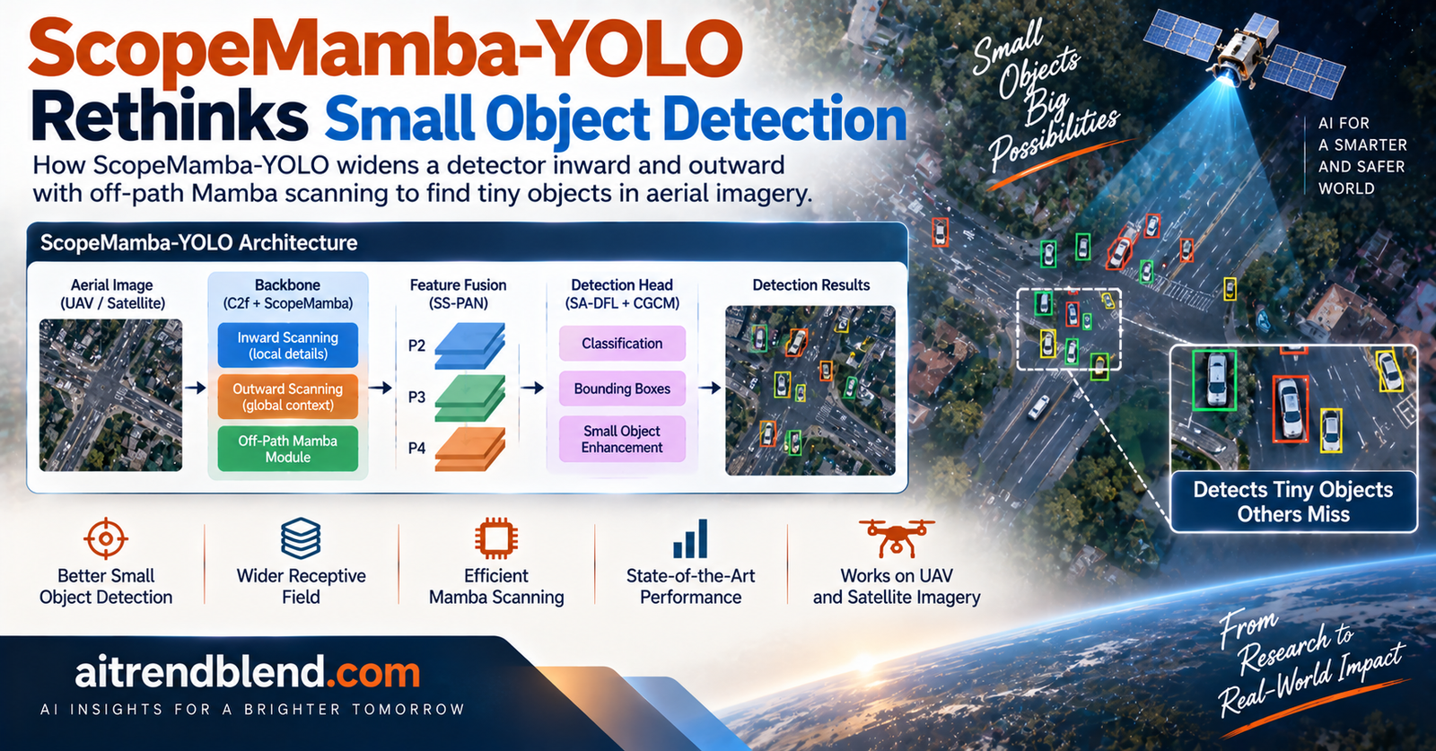
Point a camera down from a drone flying at altitude and the world turns into a field of specks. A car becomes a smudge of a dozen pixels. A pedestrian is barely a dark mark against pavement. In the VisDrone-2019 dataset that anchors this work, most annotated objects are smaller than a thirty two pixel box, and a large share fall under sixteen pixels. A detector that wants to find those objects faces a genuine contradiction, and a new paper from a team at Nanjing University of Science and Technology takes that contradiction head on.
Key points
- Tiny aerial objects demand two opposite things at once, sharper local detail and wider scene context, and most detectors can only buy one by sacrificing the other.
- ScopeMamba-YOLO runs its long range Mamba scan on a cheap side branch that re enters the main path through gates initialized to zero, so the convolutional backbone keeps full ownership of fine detail.
- Placement is the whole story. A matched experiment shows an in path scan lowers accuracy by 0.98 points, while the same off path scan raises it by 0.67 points.
- On VisDrone-2019 the small variant reaches 0.508 mAP50 with 3.57M parameters, ahead of YOLOv8s by 10.8 points while using about a third of the weights.
- A receptive field measurement backs the design, restoring roughly 61 percent of the peripheral spatial reach that pruning the deepest stage had thrown away.
The contradiction at the heart of tiny object detection
Here is where it gets interesting. A small object carries almost no appearance evidence. Its texture is sparse, its boundaries are ambiguous, and its signal to noise ratio is low. So the first instinct is to preserve resolution, because every downsampling step in a deep network erodes the little evidence a tiny target has. That pushes designers toward keeping high resolution feature maps alive deep into the network.
But correctly naming a weak signal needs more information, not less. To tell a small vehicle apart from a rooftop fixture, a network wants the surrounding scene, the roads and harbors and parking lots that give a blob its meaning. That context lives far away in the image, and reaching it normally means going deeper and coarser, which is exactly the opposite of preserving resolution. The authors call this widening the perceptual scope in two directions at once, inward toward fine grained detail and outward toward long range context. Their title turns that idea into a name, ScopeMamba-YOLO.
The common fix in aerial detection has a known side effect. Builders add a shallow stride four detection level, often called P2, to recover fine detail, and they delete the deepest stride thirty two level, called P5, to keep the model affordable. That reallocation genuinely helps tiny targets. It also quietly amputates the part of the network that used to supply broad context. The paper measures this cost directly rather than assuming it away, which is one of the more honest moves in the work.
Why not just drop a Mamba block into the backbone
State space models, and the selective Mamba variant in particular, have become the fashionable way to model long range dependencies at linear cost instead of the quadratic cost of self attention, an idea we traced in an earlier look at how Mamba is reshaping multimodal fusion. A wave of detectors has bolted Mamba scans onto backbones and necks for remote sensing. The natural question a practitioner asks is simple. If a Mamba scan gives cheap global context, why not insert it straight into the main feature path and be done?
The paper answers with an experiment rather than an opinion, and the answer is that direct insertion hurts. In a matched configuration where the only change was swapping an identity branch for an in path selective scan, mAP50 fell from 0.4949 to 0.4851, a drop of 0.98 points at unchanged computation. The interpretation is intuitive once you see it. On a shared pathway with limited channel capacity, the scan competes with the fine grained convolutions for representation, and it propagates state across feature maps where background tokens vastly outnumber the few tokens that belong to a tiny object. For a speck of a car, long range aggregation can dilute weak local evidence rather than reinforce it.
That rule is the spine of the whole architecture. The authors formalize it as an off path, zero gated, selective scanning principle. The scan runs on a low cost side branch, pooled to a quarter resolution and narrowed in channel width. It re enters the main path only through gates initialized to zero. At the very first training step the augmented network is mathematically identical to its plain convolutional skeleton, so the convolutional stream keeps full ownership of the representation, and the context branch earns its influence gradually.
How the pieces fit together
ScopeMamba-YOLO is built on the YOLOv8 skeleton and moves along a single design line that the authors describe with four verbs. Reallocate the detection scales toward high resolution, read those high resolution features cheaply, reach back out to scene context through the off path scan, and regress boxes with a budget matched to each scale. Four modules carry those verbs.
High resolution reallocation
The first step, called HRR, follows established practice. It adds the stride four P2 level, at 160 by 160 for a 640 by 640 input, and removes the stride thirty two P5 stage entirely, detecting on P2, P3, and P4 with strides four, eight, and sixteen. This is treated as an adopted prior rather than a contribution, and the paper is candid that it is not free. It drives the largest single accuracy jump in the ablation, worth 7.93 points, while cutting parameters from 11.14M to 4.14M. It also raises computation sharply, from 28.45 to 51.10 GFLOPs, because high resolution maps are expensive to process.
The AMS-Block reads anisotropic structure
Aerial scenes are full of directional structure, the long lines of vehicles along a lane, ships strung along a waterway, the geometry of parking rows. The AMS-Block replaces the bottleneck inside the C2f unit with a four branch anisotropic unit that splits channels into groups and sends two of them through horizontal and vertical strip kernels. A gate driven by global pooling blends a short strip and a long strip in each direction, and the two directional streams then modulate each other through cross gating. Because strip kernels touch about eleven pixels of extent at close to depthwise cost, the block widens the reading field while trimming parameters by roughly 24 percent and GFLOPs by about 9 percent. In the cumulative ablation it holds accuracy nearly flat, at a change of 0.07 points, while paying back much of the cost that the high resolution reallocation had added.
The CGCM brings context back without touching the main path
This is the module that repairs the damage from pruning P5. The Cascaded Global-Context Module installs two off path context stations in the backbone. From the P3 stage it pools features by a factor of four to a 20 by 20 grid, projects them down to a slim thirty two channels, normalizes, runs the four directional scan, and injects the result multiplicatively into the P4 entrance. A second station repeats the chain on a 10 by 10 grid, and importantly it reads from the already modulated P4 stage, so scene evidence accumulates along depth instead of being applied once. The multiplicative injection uses a gate written as
where the projection \(W_0\) starts at zero, so the gate spans the interval from zero to two and equals the identity at the first step. In the cumulative trajectory this station adds 0.45 points at the cost of only 0.17M parameters.
The SS-PAN neck reaches at native resolution
The neck, renamed the Selective-Scan PAN, carries two pathways. A top down pathway uses learned upsampling and directional context injection to push semantics toward the high resolution P2 feature. A bottom up pathway replaces the plain fusion unit at P3 and P4 with a C2f-SDMamba unit whose selective scan branch enters, again, through a gate initialized to zero, written as
Adding the full neck lifts accuracy by 0.63 points in the ablation. When only the bottom up scan branches are removed from the finished model, accuracy drops by 1.09 points at the small scale, which pins down how much the scanning itself contributes rather than the surrounding plumbing.
The SA-DFL head spends its regression budget by scale
Distribution Focal Loss regresses each box side as the expectation over a set of bins indexed in stride units. Standard YOLOv8 uses the same sixteen bins at every level. After the scales are reallocated, the same offset in image space corresponds to a different number of feature grid units at different strides, so a single bin budget no longer fits. The Scale-Adaptive DFL head assigns a per scale budget, twenty four bins at stride four, sixteen at stride eight, and ten at stride sixteen. Because the regression branch width scales with four times the bin count, changing the allocation also reallocates regression capacity across levels. This is the leanest module in the paper, adding only 0.008M parameters, and yet it delivers a 0.60 point gain, the largest marginal return per added parameter of any component.
The mathematics, briefly
The scan itself rests on a discretized state space recurrence. A structured model maps a one dimensional input \(x(t)\) to an output \(y(t)\) through a latent state, and after discretization with step \(\Delta\) under a zero order hold the recurrence becomes
with the discretized matrices \(\bar{\mathbf{A}} = \exp(\Delta\mathbf{A})\) and \(\bar{\mathbf{B}} = (\Delta\mathbf{A})^{-1}(\exp(\Delta\mathbf{A}) – \mathbf{I})\,\Delta\mathbf{B}\). Mamba makes the step and the input matrices depend on the input, which is what selective means, and the recurrence stays linear in sequence length. To apply this to a two dimensional feature map, the paper uses a non causal four directional variant it calls NCSSD2D, serializing the map along rows forward, rows backward, columns down, and columns up, then merging the four readings. That four way sweep gathers evidence from the whole map at a cost linear in the number of pixels, which is the property that makes a global stage affordable at all. Readers who want the wider picture on why sequence models keep displacing quadratic attention can compare this with our breakdown of what makes video vision transformers work.
What the numbers actually show
The results table is where the accuracy and parameter trade off becomes concrete. Across four scales the family stays consistently ahead of the YOLOv8 models it is built from, and it does so while carrying far fewer weights.
| Model | Params | GFLOPs | mAP50 | mAP50-95 |
|---|---|---|---|---|
| YOLOv8n | 3.00M | 8.1 | 0.341 | 0.195 |
| ScopeMamba-N | 1.01M | 15.87 | 0.439 | 0.266 |
| YOLOv8s | 11.10M | 28.7 | 0.400 | 0.238 |
| ScopeMamba-S | 3.57M | 53.69 | 0.508 | 0.314 |
| YOLOv8m | 25.90M | 79.1 | 0.435 | 0.263 |
| ScopeMamba-M | 6.48M | 92.17 | 0.526 | 0.332 |
| YOLOv8l | 43.60M | 164.9 | 0.454 | 0.279 |
| ScopeMamba-L | 9.17M | 127.78 | 0.536 | 0.337 |
The small variant is the headline. It reaches 0.508 mAP50 with 3.57M parameters, which is 10.8 points above YOLOv8s while using about 32 percent of its weights. The medium variant is arguably the more telling result, because it reaches 0.526 mAP50 with 6.48M parameters, matching the reported accuracy of the recent Mamba based detector HEdge-MamYOLO at 0.525 while using less than one third of its 20.80M parameters. Against Mamba-YOLO, which reports 0.451 mAP50 with 37.17M parameters, the gap in efficiency is stark.
The story repeats on AI-TOD, the tiny object benchmark where the mean target is only about 12.8 pixels across. The small variant improves over YOLOv8s by 4.57 points on very tiny objects, from 5.73 to 10.30, and by 4.58 points on tiny objects, from 20.97 to 25.55, while the gain on merely small objects is a more modest 0.41 points. That gradient matters, because it lines up with the stated goal. The design pays off most exactly where objects are smallest, which is what a method built for tiny targets should do.
A matched control shows in path insertion is unfavorable, while the off path formulation contributes positively. Placement, not the presence of a scan, is what turns Mamba from a liability into an asset for tiny targets. Reading of the paper’s placement experiments
The receptive field evidence
The part of the paper that lifts it above a leaderboard entry is the receptive field analysis. The authors define a Peripheral Energy Ratio, the fraction of the effective receptive field energy that lies outside the central half of the image, computed by back propagating the response of the center detection cell to the input across two hundred validation images.
The numbers tell a clean story. Unpruned YOLOv8s has a peripheral ratio of 0.147. Removing the deep P5 stage collapses it to 0.008, confirming that the popular reallocation really does concentrate attention near the image center and starve the periphery. Adding the off path context pathways then lifts the ratio back to 0.090, roughly an eleven fold increase over the pruned baseline, recovering about 61 percent of the peripheral reach that the original network had. That is a direct, physical measurement of the thing the modules were designed to fix, and it is far more persuasive than an accuracy delta alone.
Honest limitations
None of this comes for free, and the paper is refreshingly willing to say so. The most visible cost is computation. ScopeMamba-S runs at 53.69 GFLOPs against 28.7 for YOLOv8s, so the accuracy comes with almost double the arithmetic. The high resolution reallocation is the main driver, and the selective scanning in the neck adds non negligible cost on top. A practitioner deploying on a power constrained drone should weigh that carefully, because the parameter savings do not translate into proportional compute savings.
The evaluation is also bounded. Every experiment runs at 640 by 640 input, without any pretraining, and within a single YOLO style detection framework. The authors do not claim results at higher resolution, with pretrained weights, on oriented boxes, or in multi modal settings, and they name those as future directions rather than solved problems. The run to run variance is worth keeping in mind as well. The no context control was measured across three seeds at a mean of 0.5011 with a standard deviation of 0.34 points, and the full model at 0.5078 sits about 0.67 points above that mean. The gain is real and consistent in direction across scales, but the margins on individual ablation steps are small enough that the authors correctly report them as points rather than as formal significance tests.
The negative results section deserves a nod too, because it is where a lot of quiet engineering wisdom lives. Isotropic square kernels in place of the directional strips cost 1.15 points, so the anisotropy is doing real work. Stacking extra quality branches on the head gave nothing. Layering specialized localization losses such as Inner-IoU actually lowered accuracy by close to a point. Adding network depth to reallocate capacity did not match the context pathway. Reporting the experiments that failed is how you tell a design was reasoned rather than stumbled into.
Conclusion
ScopeMamba-YOLO is a careful answer to a question many recent detectors skipped over. The field rushed to put Mamba scans into vision backbones because the linear cost is attractive, but far less attention went to where the scan should sit relative to the detail carrying stream. This paper makes that placement the central object of study and shows, with a matched control, that the obvious choice of inserting the scan into the main path is the wrong one for tiny objects.
The conceptual shift is small to state and large in consequence. Treat the global operator as a modulation applied from outside the main stream, not as a replacement for part of it, and initialize its influence at zero so the convolutional network never loses its grip on fine detail during early training. That single idea threads through the backbone context stations, the neck scan branches, and the directional injection in the top down path, and it is the reason a 3.57M parameter model can outrun an 11.10M one on a hard aerial benchmark.
What makes the work transferable is that the placement rule is not tied to Mamba. Any long range operator that risks competing with local features for capacity, whether a scan, an attention block, or a large kernel, could be wrapped the same way, on a side branch behind a zero initialized gate. The receptive field diagnosis gives builders a tool as well, a way to check whether a design choice has quietly hollowed out peripheral context before that choice reaches production.
The honest remaining limitations keep expectations grounded. The compute cost is real, the tests are confined to one resolution and one detection style, and the per step margins are modest against seed variance. Those are not fatal, but they mark the edges of what has been shown. Future work on cutting context pathway latency, on higher resolution and pretrained settings, and on oriented and multi modal detection will decide whether the principle generalizes as widely as the paper hopes.
For anyone building detectors for drones, satellites, or any setting where the objects that matter are also the smallest ones on screen, the practical lesson is worth carrying forward. The same tension between local detail and scene context shows up across aerial work, from road network extraction to SAR target recognition. Widening a network inward and outward at the same time is possible, but only if the two widenings are kept in their own lanes.
Reference implementation in PyTorch
The following implementation captures the core ideas of ScopeMamba-YOLO as described in the paper, the off path zero gated context module, the anisotropic strip block, the four directional scan approximation, and the scale adaptive distributional head, with a runnable smoke test on dummy data. It is a faithful structural sketch for study, not the authors’ exact training code, and it approximates the selective scan with a lightweight recurrent form so it runs anywhere.
# scopemamba_yolo.py
# Structural reference for the ScopeMamba-YOLO ideas. Study code, not the
# authors' training pipeline. Runs a smoke test on dummy tensors at the end.

import torch
import torch.nn as nn
import torch.nn.functional as F


class ConvBNAct(nn.Module):
    """Standard conv, batchnorm, SiLU building block."""
    def __init__(self, c_in, c_out, k=3, s=1, g=1):
        super().__init__()
        p = k // 2
        self.conv = nn.Conv2d(c_in, c_out, k, s, p, groups=g, bias=False)
        self.bn = nn.BatchNorm2d(c_out)
        self.act = nn.SiLU()

    def forward(self, x):
        return self.act(self.bn(self.conv(x)))


class NCSSD2D(nn.Module):
    """Non causal four directional scan approximation.
    Serializes the map in four orders, runs a shared linear recurrence,
    and merges. A lightweight stand in for the selective state space scan."""
    def __init__(self, dim, d_state=8):
        super().__init__()
        self.dim = dim
        self.d_state = d_state
        # input dependent gate that stands in for selectivity
        self.to_gate = nn.Conv2d(dim, dim, 1)
        self.mix = nn.Conv2d(dim, dim, 1)

    def _scan_1d(self, seq, gate):
        # seq shape B, L, C. Simple gated running sum in both time directions.
        B, L, C = seq.shape
        g = torch.sigmoid(gate)
        fwd = torch.zeros_like(seq)
        acc = torch.zeros(B, C, device=seq.device, dtype=seq.dtype)
        for t in range(L):
            acc = g[:, t] * acc + (1 - g[:, t]) * seq[:, t]
            fwd[:, t] = acc
        bwd = torch.zeros_like(seq)
        acc = torch.zeros(B, C, device=seq.device, dtype=seq.dtype)
        for t in range(L - 1, -1, -1):
            acc = g[:, t] * acc + (1 - g[:, t]) * seq[:, t]
            bwd[:, t] = acc
        return fwd + bwd

    def forward(self, x):
        B, C, H, W = x.shape
        gate = self.to_gate(x)
        # rows, both directions
        row_seq = x.permute(0, 2, 3, 1).reshape(B * H, W, C)
        row_g = gate.permute(0, 2, 3, 1).reshape(B * H, W, C)
        row_out = self._scan_1d(row_seq, row_g).reshape(B, H, W, C).permute(0, 3, 1, 2)
        # columns, both directions
        col_seq = x.permute(0, 3, 2, 1).reshape(B * W, H, C)
        col_g = gate.permute(0, 3, 2, 1).reshape(B * W, H, C)
        col_out = self._scan_1d(col_seq, col_g).reshape(B, W, H, C).permute(0, 3, 2, 1)
        return self.mix(row_out + col_out)


class CGCM(nn.Module):
    """Cascaded Global-Context Module. Off path scan, injected through a
    zero initialized tanh gate so it is identity at init."""
    def __init__(self, dim, pool=4, ctx_dim=32, d_state=8):
        super().__init__()
        self.pool = pool
        self.down = nn.Conv2d(dim, ctx_dim, 1)
        self.norm = nn.GroupNorm(1, ctx_dim)
        self.scan = NCSSD2D(ctx_dim, d_state)
        self.up = nn.Conv2d(ctx_dim, dim, 1)
        # zero initialized projection makes the gate the identity at step zero
        self.gate_proj = nn.Conv2d(dim, dim, 1)
        nn.init.zeros_(self.gate_proj.weight)
        nn.init.zeros_(self.gate_proj.bias)

    def forward(self, x):
        B, C, H, W = x.shape
        g = F.adaptive_avg_pool2d(x, (H // self.pool, W // self.pool))
        g = self.up(self.scan(self.norm(self.down(g))))
        g = F.interpolate(g, size=(H, W), mode="bilinear", align_corners=False)
        # F_hat = F * (1 + tanh(W0 g)), identity when W0 = 0
        return x * (1 + torch.tanh(self.gate_proj(g)))


class AMSBlock(nn.Module):
    """Adaptive Multi scale Strip block. Four channel groups, anisotropic
    strip branches with a pooled gate, cross directional gating, residual."""
    def __init__(self, dim):
        super().__init__()
        c = dim // 4
        self.c = c
        self.local = nn.Conv2d(c, c, 3, 1, 1, groups=c)
        self.h_short = nn.Conv2d(c, c, (1, 5), 1, (0, 2), groups=c)
        self.h_long = nn.Conv2d(c, c, (1, 11), 1, (0, 5), groups=c)
        self.v_short = nn.Conv2d(c, c, (5, 1), 1, (2, 0), groups=c)
        self.v_long = nn.Conv2d(c, c, (11, 1), 1, (5, 0), groups=c)
        self.gate_h = nn.Conv2d(c, c, 1)
        self.gate_v = nn.Conv2d(c, c, 1)
        self.cross_h = nn.Conv2d(c, c, 1)
        self.cross_v = nn.Conv2d(c, c, 1)
        self.fuse = nn.Conv2d(dim, dim, 1)

    def forward(self, x):
        x1, x2, x3, x4 = torch.split(x, self.c, dim=1)
        f_local = self.local(x1)
        a_h = torch.sigmoid(self.gate_h(F.adaptive_avg_pool2d(x2, 1)))
        f_h = a_h * self.h_short(x2) + (1 - a_h) * self.h_long(x2)
        a_v = torch.sigmoid(self.gate_v(F.adaptive_avg_pool2d(x3, 1)))
        f_v = a_v * self.v_short(x3) + (1 - a_v) * self.v_long(x3)
        # cross directional gating, each stream modulates the other
        fh = f_h * torch.sigmoid(self.cross_v(f_v))
        fv = f_v * torch.sigmoid(self.cross_h(f_h))
        out = torch.cat([f_local, fh, fv, x4], dim=1)
        return x + self.fuse(out)


class SADFLHead(nn.Module):
    """Scale-Adaptive DFL head. Each level gets its own bin budget K,
    and the regression branch width scales with 4 * K."""
    def __init__(self, dims, n_classes=10, ks=(24, 16, 10)):
        super().__init__()
        self.ks = ks
        self.n_classes = n_classes
        self.cls_heads = nn.ModuleList()
        self.reg_heads = nn.ModuleList()
        for dim, k in zip(dims, ks):
            c_reg = max(16, (dim // 4), 4 * k)
            self.cls_heads.append(nn.Sequential(
                ConvBNAct(dim, dim, 3), nn.Conv2d(dim, n_classes, 1)))
            self.reg_heads.append(nn.Sequential(
                ConvBNAct(dim, c_reg, 3), nn.Conv2d(c_reg, 4 * k, 1)))

    def _expect(self, reg, k):
        B, _, H, W = reg.shape
        reg = reg.view(B, 4, k, H, W)
        p = F.softmax(reg, dim=2)
        bins = torch.arange(k, device=reg.device, dtype=reg.dtype).view(1, 1, k, 1, 1)
        return (p * bins).sum(dim=2)  # B, 4, H, W distances in stride units

    def forward(self, feats):
        outs = []
        for f, cls_h, reg_h, k in zip(feats, self.cls_heads, self.reg_heads, self.ks):
            logits = cls_h(f)
            dist = self._expect(reg_h(f), k)
            outs.append((logits, dist))
        return outs


class ScopeMambaYOLO(nn.Module):
    """Compact structural assembly. Backbone with HRR scales P2 P3 P4,
    AMS blocks, off path CGCM context, and a scale adaptive head."""
    def __init__(self, width=(64, 128, 256), n_classes=10):
        super().__init__()
        w2, w3, w4 = width
        self.stem = nn.Sequential(ConvBNAct(3, w2, 3, 2), ConvBNAct(w2, w2, 3, 2))  # stride 4, P2
        self.p2 = AMSBlock(w2)
        self.down3 = ConvBNAct(w2, w3, 3, 2)  # stride 8, P3
        self.p3 = AMSBlock(w3)
        self.ctx3 = CGCM(w3)
        self.down4 = ConvBNAct(w3, w4, 3, 2)  # stride 16, P4
        self.p4 = AMSBlock(w4)
        self.ctx4 = CGCM(w4)
        self.head = SADFLHead([w2, w3, w4], n_classes, ks=(24, 16, 10))

    def forward(self, x):
        f2 = self.p2(self.stem(x))
        f3 = self.p3(self.down3(f2))
        f3 = self.ctx3(f3)  # off path context injected before deepening
        f4 = self.p4(self.down4(f3))
        f4 = self.ctx4(f4)  # cascaded, reads the already modulated stage
        return self.head([f2, f3, f4])


def dfl_loss(pred_dist, target_dist, k):
    """Distribution focal style regression on expected distances."""
    return F.l1_loss(pred_dist, target_dist.clamp(0, k - 1))


def smoke_test():
    torch.manual_seed(0)
    model = ScopeMambaYOLO(width=(32, 64, 128), n_classes=10)
    x = torch.randn(2, 3, 128, 128)  # small input for a fast check
    outs = model(x)
    for i, (logits, dist) in enumerate(outs):
        print(f"level {i} cls {tuple(logits.shape)} reg {tuple(dist.shape)}")
    # verify the zero gate is identity at init on one context module
    z = torch.randn(1, 64, 32, 32)
    ctx = CGCM(64)
    diff = (ctx(z) - z).abs().max().item()
    print(f"context identity error at init {diff:.2e}")
    n_params = sum(p.numel() for p in model.parameters())
    print(f"parameter count {n_params/1e6:.3f} M")


if __name__ == "__main__":
    smoke_test()
Running the smoke test prints the three detection level shapes, confirms the context module behaves as the identity at initialization by reporting a near zero difference, and reports the parameter count. The identity check is the important one, because it verifies the zero gated property that the whole design depends on.
Frequently asked questions
What problem does ScopeMamba-YOLO solve?
It targets the detection of very small objects in drone and remote sensing images, where tiny targets need both sharper local detail and wider scene context at the same time. The design widens the network in both directions without letting one goal cancel the other.
Why does the paper avoid putting the Mamba scan in the main path?
A matched experiment showed that inserting the selective scan directly into the backbone lowered accuracy by 0.98 points at equal computation, because the scan competes with fine grained features and spreads state over background heavy maps. Placing it on a side branch behind a gate initialized to zero avoided that harm and added 0.67 points instead.
How much better is it than the YOLOv8 baseline?
On VisDrone-2019 the small variant reached 0.508 mAP50 with 3.57M parameters against 0.400 for YOLOv8s at 11.10M, an improvement of 10.8 points using about a third of the weights. Gains held across the nano, medium, and large variants as well.
What is the Peripheral Energy Ratio and why does it matter?
It measures how much of a detector’s effective receptive field lies outside the image center. Removing the deep stage dropped it from 0.147 to 0.008, and the off path context pathways lifted it back to 0.090, showing that the modules restored roughly 61 percent of the peripheral reach that pruning had removed.
What are the main limitations?
The accuracy comes with higher computation, about 53.69 GFLOPs for the small model against 28.7 for YOLOv8s. The evaluation is also limited to 640 by 640 input, no pretraining, and YOLO style detection, and per step ablation margins are small relative to the measured seed variance of 0.34 points.
Can the placement idea transfer to other detectors?
Yes. The rule of running a long range operator on a side branch behind a zero initialized gate is not specific to Mamba and could wrap attention blocks or large kernel operators too, along with the receptive field diagnostic used to check for lost context.
Read the full paper and explore the method in the authors’ own words.
Read the paper on arXiv