
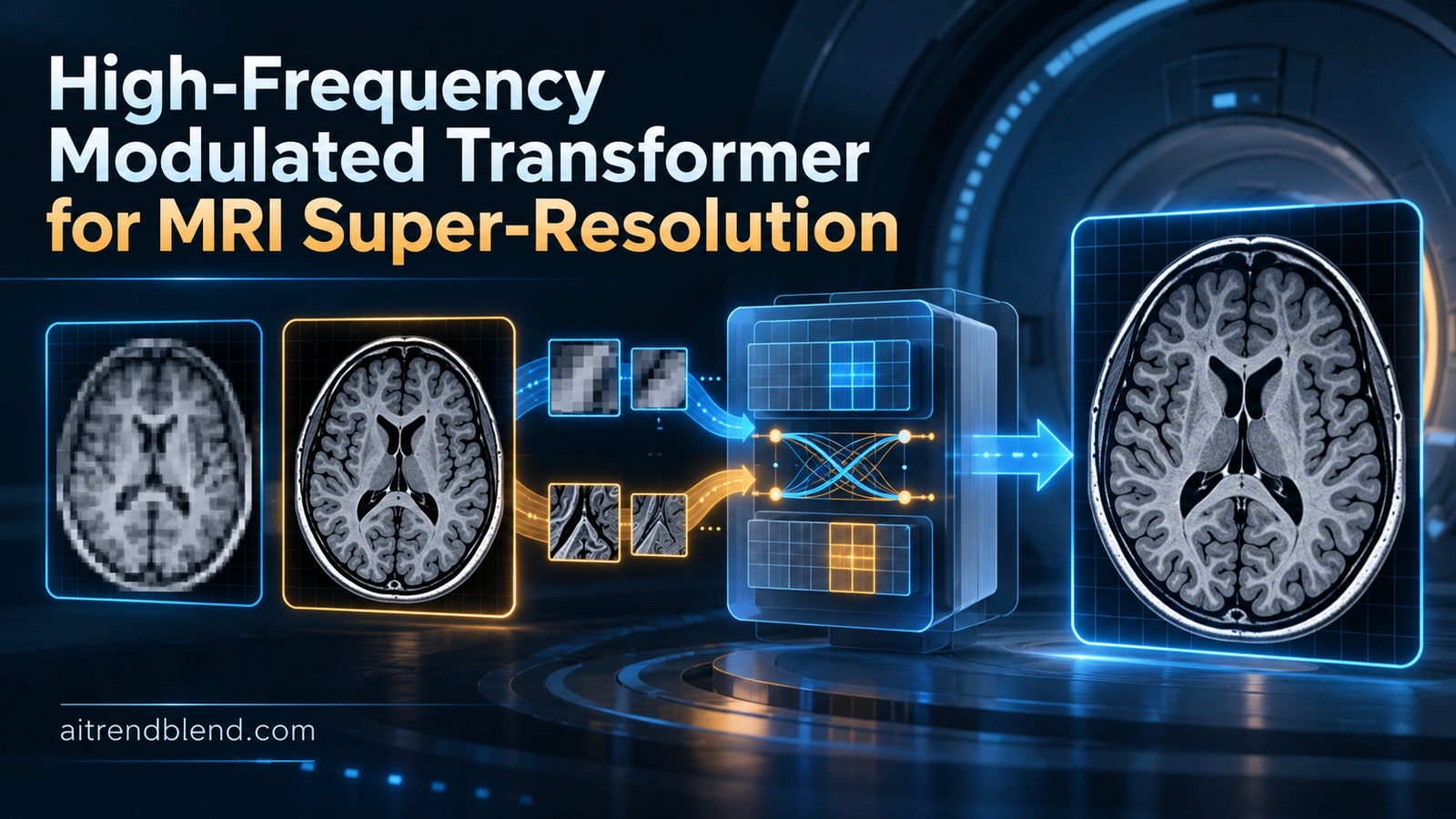
Inside an oncology department preparing a patient for image-guided adaptive radiation therapy, or inside a musculoskeletal clinic evaluating a torn meniscus, lying motionless inside a magnetic resonance bore for thirty minutes is an exhausting ordeal. Acquiring crisp, high-resolution T2-weighted brain volumes or fat-suppressed proton density knee scans takes prolonged scan times governed by the physical laws of k-space sampling, while companion sequences such as standard proton density scans finish in a fraction of the time. Juncheng Li, Hanhui Yang, Qiaosi Yi, Minhua Lu, Jun Shi, and Tieyong Zeng at Shanghai University, The Chinese University of Hong Kong, The Hong Kong Polytechnic University, and Shenzhen University developed the High-Frequency Modulated Transformer (HFMT) to transfer sharp anatomical edges from fast reference scans into heavily undersampled target scans using just 2.5 million parameters.
Key Research Takeaways
- HFMT processes multi-contrast MRI super-resolution at low spatial resolution first by downsampling the reference scan, slashing computation to 39.67 GFlops (compared to 677.58 GFlops in MINet and 462.55 GFlops in SANet) before restoring full-resolution reference details at the final stage.
- An Enhance, Matching, and Extraction Block (EMEB) isolates high-frequency edge residuals via average-pooling subtraction and uses a three-stage cosine similarity patch matcher to align relevant reference textures with the target contrast.
- Within each Cross Fusion Residual Group (CFRG), a Rectangle Window Transformer Block (RWTB) pairs horizontal (\(4 \times 16\)) and vertical (\(16 \times 4\)) attention windows with a lightweight 0.2M-parameter High-Frequency Fusion Block (HFFB) that computes \(C \times C\) channel-wise cross-attention instead of expensive \(HW \times HW\) spatial maps.
- At \(4\times\) acceleration (retaining only 6.25 percent of central k-space), HFMT achieves 31.02 dB PSNR and 0.639 SSIM on FastMRI knee scans and 38.00 dB PSNR and 0.971 SSIM on IXI brain scans, outperforming 104M-parameter CANM-Net (30.84 dB and 37.97 dB) and 43M-parameter DANCE (30.91 dB).
- Removing the final Symmetric Refined Fusion Block (SRFB) causes a 6.93 dB PSNR collapse on IXI \(4\times\) brain reconstructions (dropping from 38.002 dB to 31.069 dB), proving that recovering lost full-resolution reference frequencies after upsampling is essential.
This article analyzes peer-reviewed medical imaging and signal processing research published in IEEE Transactions on Medical Imaging and is provided strictly for informational and educational purposes. It does not constitute medical advice, clinical diagnosis, radiology protocol guidance, or treatment recommendations. Clinical acquisition and diagnostic interpretation of Magnetic Resonance Imaging sequences must always be performed and verified by qualified radiologists, medical physicists, and licensed healthcare professionals.
Why k-Space Undersampling Blurs Clinical MRI and How Multi-Contrast Priors Help
The problem runs deeper than it first appears. Magnetic Resonance Imaging (MRI) is indispensable for radiation-free soft tissue diagnostics and image-guided adaptive radiation therapy, yet every scan is bound by the Nyquist sampling theorem formulated in 1928. Because an MR scanner acquires raw spatial-frequency measurements line by line in k-space, reconstructing a high-resolution image free of aliasing requires dense phase-encoding steps that keep patients inside the magnet for extended periods. Prolonged scan durations increase patient discomfort, trigger claustrophobia, reduce scanner throughput, and invite involuntary motion artifacts.
In routine clinical practice, physicists accelerate acquisition by subsampling k-space, keeping only the central low-frequency region while zeroing out peripheral high-frequency data points. For a \(2\times\) spatial acceleration factor, only the central 25 percent of k-space points are retained, and for a \(4\times\) acceleration factor, the scanner captures a mere 6.25 percent of the central k-space grid before applying an inverse Fourier transform. Because the center of k-space encodes bulk tissue contrast and overall brightness while the periphery encodes sharp anatomical boundaries, cortical sulci, cartilage interfaces, and fine vessel walls, clearing the outer 75 to 93.75 percent of k-space yields a low-resolution image stripped of high-frequency diagnostic detail.
Here is where clinical workflow offers a natural shortcut. Modern MR protocols almost never acquire a single isolated sequence. A brain exam pairs T1-weighted images (T1WI), which capture crisp anatomical morphology, with T2-weighted images (T2WI), which highlight peritumoral edema and inflammation. Similarly, a musculoskeletal knee exam pairs Proton Density (PD) sequences with Fat-Suppressed Proton Density-Weighted Images (PDFS or FS-PDWI). Crucially, these sequences take very different amounts of time to acquire. A standard PD volume is rapid and straightforward to collect, whereas a PDFS or T2WI volume requires longer repetition times and fat-saturation pulses.
If you run a Sobel edge detector across an aligned pair of PD and PDFS knee images from the exact same patient, a striking physical property emerges. Even though their grayscale intensity profiles and tissue contrasts look completely different, their high-frequency edge maps—the sharp boundaries, corners, meniscal margins, and trabecular bone textures—are nearly identical. Multi-Contrast Super-Resolution (MCSR) exploits this redundancy by using a fast, fully sampled reference contrast (such as PD) to guide the super-resolution recovery of a heavily undersampled target contrast (such as PDFS or T2WI). For readers following our coverage in the AI for medical imaging and healthcare hub, MCSR represents one of the cleanest examples of physics-informed cross-modal synergy in medical vision.
Background and Prior Work in Reference-Based MRI Super-Resolution
Early attempts at multi-contrast MRI restoration relied on hand-crafted statistical priors. Rousseau et al. introduced non-local patch weights across intermodality priors in 2010, while Zheng et al. estimated local regression weights and gradient-guided edge priors from high-resolution reference scans to interpolate low-resolution target pixels. When convolutional neural networks (CNNs) entered the field, Zeng et al. proposed SCSR to perform simultaneous single-contrast and multi-contrast super-resolution via direct input concatenation, and Lyu et al. demonstrated that concatenating multi-contrast representations in deeper feature space outperforms raw pixel stacking. Later CNN architectures such as MINet by Feng et al. introduced multi-stage integration, while SANet explored separable attention across high-intensity and low-intensity regions.
Despite steady gains, purely convolutional backbones struggle with two fundamental limitations. First, local \(3 \times 3\) kernels have restricted receptive fields that cannot capture long-range anatomical symmetry across an entire brain hemisphere or knee joint. Second, naive concatenation treats every reference pixel equally, even when local contrast inversions or registration shifts make parts of the reference scan unhelpful. Vision Transformers addressed the receptive field bottleneck by introducing self-attention and cross-attention, a shift we also examined in our review of attention mechanisms for medical image segmentation. Models such as MTrans by Feng et al. (86.1M parameters), McMRSR by Li et al. (3.9M parameters), WavTrans by Li et al., CANM-Net by Chen et al. (104M parameters), MAPANet by Liu et al. (5.9M parameters), and DANCE by Chen et al. (43M parameters) applied multi-scale Swin blocks, wavelet projections, or deformable neighborhood aggregation to fuse reference and target streams.
Yet existing Transformer MCSR architectures suffer from two severe engineering blind spots. First, most models immediately upsample the low-resolution target scan to full resolution at the network entrance and compute spatial cross-attention of size \(HW \times HW\), ballooning memory consumption and parameter counts past 80 to 100 million. Second, standard self-attention acts as a low-pass spatial filter that smooths out high-frequency edges unless explicitly modulated by frequency priors—a phenomenon demonstrated in frequency separation networks by Li et al., Frequency-based Enhancement Blocks (FEB) by Behjati et al., Edge Attention MRI (EAMRI) by Yang et al., and Feature Modulation Transformers by Li et al. In their IEEE Transactions on Medical Imaging paper introducing HFMT, Li and colleagues bridge both gaps simultaneously.
Inside the High-Frequency Modulated Transformer Architecture
Think about how much computation is wasted when a network upsamples a \(64 \times 64\) or \(80 \times 80\) low-resolution MRI slice to \(256 \times 256\) or \(320 \times 320\) before running a single transformer block. Interpolating early not only multiplies the pixel count by 16 under \(4\times\) enlargement, it also bakes bicubic interpolation errors into every subsequent layer. HFMT flips that design on its head by feeding the network three distinct inputs: the low-resolution target contrast image \(lr\), the full-resolution reference contrast image \(ref\), and a bicubic-downsampled version of the reference image \(ref_{lr}\) matched to the exact spatial dimensions of \(lr\).
An initial shallow convolutional Head extracts 72-channel feature maps \(f_{lr}\), \(f_{reflr}\), and \(f_{ref}\) from these three inputs. All heavy feature extraction, patch matching, and transformer cross-fusion happen at the compact low resolution using \(f_{lr}\) and \(f_{reflr}\). Specifically, \(f_{reflr}\) passes through the Enhance, Matching, and Extraction Block (EMEB) to amplify its high-frequency priors and align them spatially with \(f_{lr}\). The resulting enhanced reference features and \(f_{lr}\) then traverse three sequential Cross Fusion Residual Groups (CFRGs) connected by a global long-skip residual path before an upsampling layer restores full target resolution \(f_{up}\). Finally, because downsampling \(ref\) to \(ref_{lr}\) inevitably discards ultra-fine native edges, the Symmetric Refined Fusion Block (SRFB) fuses \(f_{up}\) with the full-resolution shallow reference features \(f_{ref}\) to render the final super-resolved scan.
By running patch matching and three Cross Fusion Residual Groups at low resolution on \(f_{reflr}\) and deferring full-resolution reference integration to the lightweight Symmetric Refined Fusion Block at the very end, HFMT cuts computational complexity to 39.67 GFlops—nearly 17 times fewer operations than MINet (677.58 GFlops) and over 11 times fewer than SANet (462.55 GFlops)—while outperforming 104M-parameter CANM-Net with just 2.5M parameters.
Enhance, Matching, and Extraction Block (EMEB)
EMEB prepares the downsampled reference features \(f_{reflr}\) through two sequential sub-modules: the Enhancement Block (EB) and the Matching and Extraction Block (MEB). Inside the Enhancement Block, an incoming feature tensor \(X\) is split evenly along the channel dimension into two halves, \(X_1\) and \(X_2\). While \(X_2\) passes through a standard \(3 \times 3\) convolution to preserve baseline structural context, \(X_1\) undergoes average pooling followed by bicubic upsampling to produce a low-pass smoothed representation \(X_s\). Subtracting \(X_s\) from \(X_1\) isolates the pure high-frequency residual \(X_h\), which is then passed through a convolutional layer and added back to \(X_1\) before concatenating both branches.
Once EB has amplified the high-frequency edges in \(f_{reflr}\), the Matching and Extraction Block (MEB)—adapted from the MASA-SR algorithm by Lu et al. for multi-contrast MRI without requiring a high-resolution target image—eliminates redundant reference regions and aligns reference patches to the target feature map \(f_{lr}\) in three stages:
- Stage 1 (Block-Level Coarse Search): The target feature map \(F_{lr}\) is partitioned into non-overlapping \(8 \times 8\) blocks. Simultaneously, the enhanced reference feature map \(F_{reflr}\) is unfolded into overlapping \(3 \times 3\) patches. For each \(8 \times 8\) block in \(F_{lr}\), the algorithm extracts its central \(3 \times 3\) patch, computes the cosine similarity against all \(3 \times 3\) patches across \(F_{reflr}\), identifies the highest-scoring reference coordinate, and crops a \(13 \times 13\) local neighborhood around that best match to form a paired candidate block \((B_{lr}^i, B_{reflr}^i)\).
- Stage 2 (Dense Intra-Block Patch Matching): Within each matched pair \((B_{lr}^i, B_{reflr}^i)\), both blocks are unfolded into overlapping \(3 \times 3\) patches. Assuming \(K\) patches in \(B_{lr}^i\), cosine similarity is computed between every target patch in \(B_{lr}^i\) and every candidate patch inside the \(13 \times 13\) reference block \(B_{reflr}^i\). The highest similarity score and its corresponding patch index are recorded in vectors \(S^i \in \mathbb{R}^K\) and \(I^i \in \mathbb{N}^K\).
- Stage 3 (Similarity-Weighted Reassignment and Folding): For the \(j\)-th patch position inside block \(i\), the matcher retrieves the \(I_j^i\)-th patch from \(B_{reflr}^i\), multiplies it by its confidence weight \(S_j^i\), and folds all reassembled blocks back into a spatially aligned, high-frequency-enriched reference feature map \(F_{reflr}\).
Cross Fusion Residual Group (CFRG) and Successive Modulation
The core backbone of HFMT consists of three stacked Cross Fusion Residual Groups (CFRGs), each operating on 72 feature channels. Inside every CFRG, the target features \(f_{lr}\) split into two parallel paths. The upper path enters a Rectangle-Window Transformer Block (RWTB) with 6 attention heads to capture long-range global context \(f_{global}\) across horizontal (\(4 \times 16\)) and vertical (\(16 \times 4\)) rectangular windows, which cover a wider directional receptive field than square Swin windows. The lower path passes \(f_{lr}\) through another Enhancement Block (EB) to amplify the target contrast’s own native high-frequency edges, producing \(f_{lr}’\).
Why enhance high frequencies in both \(f_{reflr}\) and \(f_{lr}’\)? Because while reference and target sequences share most anatomical boundaries, modality-specific tissue contrasts still differ in certain lesions and fluid compartments. HFMT resolves this discrepancy through a High-Frequency Successive Fusion Strategy (HFSFS) using two cascaded High-Frequency Fusion Blocks (HFFBs). The first HFFB modulates \(f_{global}\) using the aligned reference priors \(f_{reflr}\), injecting sharp external edges. Immediately afterward, the second HFFB modulates that intermediate output using the target’s own high-frequency features \(f_{lr}’\), shifting the feature distribution back toward the target contrast before a \(3 \times 3\) convolution and a group-level residual skip connection complete the CFRG.
Mathematical Formulations of High-Frequency Modulation and Fusion
To see how each module operates without computational bloat, let us walk through the exact equations governing HFMT. First, inside the Enhancement Block (EB), high-frequency isolation and amplification on the upper channel split \(X_1\) are defined by Equations 1 and 2 of the paper.
Here, \(X_s = \text{Upsample}_{\text{bicubic}}(\text{AvgPool}(X_1))\) represents the low-frequency smoothed feature map, and \(X_h\) captures the high-frequency difference before a learned convolution refines and adds those edges back to \(X_1\).
Next, inside the Rectangle-Window Transformer Block (RWTB), an input tensor \(X \in \mathbb{R}^{H \times W \times C}\) is partitioned into \(N_1\) horizontal windows (\(\text{H-Rwin}\) of size \(4 \times 16\)) and \(N_2\) vertical windows (\(\text{V-Rwin}\) of size \(16 \times 4\)). For the \(j\)-th window \(X_j \in \mathbb{R}^{(h \times w) \times C}\) with query \(Q_j\), key \(K_j\), value \(V_j\), head dimension \(d\), and dynamic relative position encoding \(B\) from CrossFormer++, local window attention and multi-head concatenation follow Equations 3, 4, and 5.
Inside each High-Frequency Fusion Block (HFFB), rather than computing an \(HW \times HW\) spatial attention matrix, HFMT adopts transposed channel-wise cross-attention inspired by Restormer. Specifically, the high-frequency feature map (\(f_{reflr}\) in the first HFFB, or \(f_{lr}’\) in the second HFFB) passes through \(\text{DConv}\) (a \(1 \times 1\) point-wise convolution followed by a \(3 \times 3\) depth-wise convolution) and is reshaped into a query matrix \(Q \in \mathbb{R}^{C \times HW}\). Meanwhile, the LayerNormed global feature tensor \(f_{global}\) passes through separate \(\text{DConv}\) layers and is reshaped into key \(K \in \mathbb{R}^{C \times HW}\) and value \(V \in \mathbb{R}^{HW \times C}\). Their interaction generates a compact \(C \times C\) channel attention map (\(72 \times 72\)), supplemented by a parallel \(3 \times 3\) local convolution branch on \(f_{global}\) and a Feed-Forward Network (\(\text{FFN}\)).
Finally, after the third CFRG output is added to the initial shallow feature \(f_{lr}\) and upsampled to the target high resolution \(f_{up}\), the Symmetric Refined Fusion Block (SRFB) computes bidirectional residual differences against the full-resolution shallow reference features \(f_{ref}\) via Equations 6 and 7 before concatenating both refined streams.
This symmetric cross-subtraction explicitly isolates what \(f_{ref}\) contains that \(f_{up}\) missed during low-resolution processing (\(Res_{ref}\)), and what target-specific contrast structures \(f_{up}\) possesses that differ from the reference scan (\(Res_{up}\)).
Experimental Benchmarks on FastMRI Knee and IXI Brain Datasets
The authors evaluated HFMT across two gold-standard public MRI repositories under both \(2\times\) (25 percent central k-space retained) and \(4\times\) (6.25 percent central k-space retained) frequency-domain truncation. First, on the FastMRI single-coil knee dataset established by Facebook AI Research and NYU Langone Health, 227 aligned volume pairs of Proton Density (PD as reference) and Fat-Suppressed PD-Weighted (FS-PDWI as target) scans cropped to \(320 \times 320\) in k-space were used for training, with 24 aligned volume pairs for validation. Second, on the London multi-hospital IXI brain dataset, 19,140 aligned slices of PD (reference) and T2-weighted (target) scans cropped to \(256 \times 256\) were used for training and 2,592 slices for testing. All models were trained for up to 50 epochs with batch size 4, \(L_1\) loss, and Adam optimizer (\(lr = 2 \times 10^{-4}\)) on an NVIDIA Quadro RTX8000 GPU.
| Method & Year | Category | Params (M) ↓ | FastMRI 2× PSNR / SSIM ↑ | FastMRI 4× PSNR / SSIM ↑ | IXI Brain 2× PSNR / SSIM ↑ | IXI Brain 4× PSNR / SSIM ↑ |
|---|---|---|---|---|---|---|
| MSRN (2018) | SISR (CNN) | 6.3 M | 31.56 dB / 0.711 | 29.46 dB / 0.612 | 38.91 dB / 0.980 | 30.55 dB / 0.919 |
| SCSR (2018) | SISR / MCSR | — | 31.58 dB / 0.716 | 29.48 dB / 0.619 | 38.94 dB / 0.981 | 30.58 dB / 0.921 |
| RCAN (2018) | SISR (CNN) | 15.59 M | 31.93 dB / 0.714 | 30.04 dB / 0.615 | — | — |
| MINet (2021) | MCSR (CNN) | 6.9 M | 32.12 dB / 0.719 | 30.75 dB / 0.630 | 42.82 dB / 0.986 | 37.66 dB / 0.967 |
| MTrans (2022) | MCSR (Transformer) | 86.1 M | 31.90 dB / 0.711 | 30.31 dB / 0.615 | 41.66 dB / 0.977 | 35.82 dB / 0.951 |
| McMRSR (2022) | MCSR (Transformer) | 3.9 M | 32.15 dB / 0.720 | 30.77 dB / 0.630 | 42.97 dB / 0.986 | 37.84 dB / 0.968 |
| CANM-Net (2023) | MCSR (Transformer) | 104.0 M | 32.16 dB / 0.720 | 30.84 dB / 0.635 | 43.15 dB / 0.986 | 37.97 dB / 0.970 |
| SANet (2024) | MCSR (Attention) | 7.5 M | 32.01 dB / 0.719 | 30.60 dB / 0.627 | 42.65 dB / 0.985 | 36.96 dB / 0.965 |
| MAPANet (2024) | MCSR (Attention) | 5.9 M | 32.21 dB / 0.720 | 30.92 dB / 0.637 | — | — |
| DANCE (2025) | MCSR (Deformable) | 43.0 M | 32.19 dB / 0.722 | 30.91 dB / 0.636 | — | — |
| HFMT (Ours, 2025) | MCSR (HF Transformer) | 2.5 M | 32.23 dB / 0.723 | 31.02 dB / 0.639 | 43.19 dB / 0.987 | 38.00 dB / 0.971 |
Look at the parameter efficiency in Table 1 above. MTrans uses 86.1 million parameters and CANM-Net uses 104 million parameters—over 41 times larger than HFMT—yet HFMT beats both of them across every single scale and dataset, reaching 31.02 dB PSNR and 0.639 SSIM on FastMRI \(4\times\) and 38.00 dB PSNR and 0.971 SSIM on IXI \(4\times\). Even against the 2025 deformable neighborhood network DANCE (43M parameters, 30.91 dB on FastMRI \(4\times\)) and MAPANet (5.9M parameters, 30.92 dB), HFMT holds a clear lead at 2.5M parameters. Furthermore, in a direct comparison against the original MASA-SR architecture (4.0M parameters) adapted to \(4\times\) MCSR in Table V of the paper, MASA-SR scores 30.84 dB / 0.631 on FastMRI and 33.99 dB / 0.952 on IXI, whereas HFMT jumps by +4.01 dB on IXI to 38.00 dB / 0.971.
“Unlike most common methods that upsample the low-resolution image to the same size as the reference image before performing subsequent operations, we choose to downsample the reference image to the same resolution as the low-resolution input since this method can greatly reduce computational overhead and will not introduce unnecessary error information.”
Juncheng Li, Hanhui Yang, Qiaosi Yi, Minhua Lu, Jun Shi, and Tieyong Zeng, IEEE Transactions on Medical Imaging (2025)
Computational Complexity and Component Ablation Studies
To quantify hardware efficiency on \(320 \times 320\) images under \(4\times\) enlargement (Table IV of the paper), the authors measured parameter count, GFlops (GMac), and inference latency per iteration, alongside systematic ablation experiments across all four core modules (Table III).
| Experiment / Variant | Configuration Description | Params / GFlops / Latency | IXI 4× PSNR (dB) / SSIM ↑ | FastMRI 4× PSNR (dB) / SSIM ↑ |
|---|---|---|---|---|
| MINet Baseline | Multi-stage CNN integration at full resolution | 6.9M / 677.58G / 3.47 s | 37.660 / 0.9670 | 30.750 / 0.6300 |
| SANet Baseline | Separable attention network | 7.5M / 462.55G / 2.20 s | 36.960 / 0.9650 | 30.600 / 0.6270 |
| MASA Baseline | Reference matching and spatial adaptation | 4.0M / 140.74G / 2.15 s | 33.990 / 0.9520 | 30.840 / 0.6310 |
| HFMT-low (Ablation 1a) | Replaces EB with AvgPool + bicubic smoothing (\(X_s\) only) | — | 35.704 / 0.9629 | 30.917 / 0.6338 |
| HFMT-ori (Ablation 1b) | Removes EB completely (no high-frequency amplification) | — | 37.792 / 0.9701 | 30.974 / 0.6373 |
| CNN-simple (Ablation 2a) | Replaces HFFB with simple concatenation + \(3\times 3\) Conv | — | 37.435 / 0.9680 | 30.924 / 0.6363 |
| CNN-ca (Ablation 2b) | Replaces HFFB with CBAM channel attention | — | 37.938 / 0.9702 | 30.961 / 0.6372 |
| HFMT-ref (Ablation 3) | Removes second HFFB in CFRG (uses reference HF only) | — | 37.918 / 0.9703 | 30.967 / 0.6372 |
| HFMT-simple (Ablation 4a) | Removes SRFB completely (no full-resolution \(f_{ref}\)) | — | 31.069 / 0.9280 | 30.860 / 0.6310 |
| HFMT-cnn (Ablation 4b) | Replaces SRFB with a single \(3\times 3\) convolution | — | 35.646 / 0.9598 | 30.888 / 0.6325 |
| HFMT Full (Ours) | Complete EMEB + 3× CFRG (RWTB + 2× HFFB) + SRFB | 2.5M / 39.67G / 1.51 s | 38.002 / 0.9705 | 31.025 / 0.6386 |
The ablation numbers in Table 2 expose why each design choice matters. First, smoothing out high frequencies in `HFMT-low` causes a 2.088 dB drop on IXI compared to `HFMT-ori` (35.704 dB vs 37.792 dB), while adding the Enhancement Block in full `HFMT` boosts IXI PSNR by another +0.21 dB to 38.002 dB. Second, replacing the 0.2M-parameter HFFB cross-attention module with simple concatenation (`CNN-simple`) loses 0.567 dB on IXI. Third, dropping the target-contrast high-frequency modulation branch (`HFMT-ref`) reduces PSNR on both IXI and FastMRI, confirming that successive modulation across both contrasts outperforms reference-only guidance. Most dramatically, omitting the Symmetric Refined Fusion Block (`HFMT-simple`) causes IXI PSNR to plummet by 6.933 dB (from 38.002 dB down to 31.069 dB), and replacing SRFB with a plain convolution (`HFMT-cnn`) still loses 2.356 dB.
Clinical Translation Gap Between k-Space Simulation and Hospital Scanners
Achieving 38.00 dB PSNR on retrospective brain slices and 31.02 dB on knee volumes with a 2.5M-parameter network is an impressive feat of compact model engineering, much like the parameter-efficient tuning strategies we covered in Rein++ domain generalization for vision foundation models. However, deploying a multi-contrast super-resolution model inside a hospital PACS or scanner reconstruction console introduces clinical translation hurdles that go beyond benchmark tables.
First, consider inter-scan patient motion and spatial misregistration. In both the FastMRI and IXI experiments, the reference PD volume and the target FS-PDWI or T2 volume are pre-aligned. In a live radiology suite, the reference scan and the target scan are acquired sequentially several minutes apart. If a patient shifts their knee by three millimeters, coughs, or tilts their head between the fast PD sequence and the accelerated T2 sequence, the full-resolution feature map \(f_{ref}\) fed into the final Symmetric Refined Fusion Block (SRFB) will no longer align pixel-for-pixel with the upsampled target \(f_{up}\). While the Matching and Extraction Block (MEB) searches a \(13 \times 13\) window at low resolution to handle minor shifts in \(f_{reflr}\), SRFB performs direct pixelwise subtraction (\(\text{Conv}(f_{ref}) – f_{up}\)) at full resolution without deformable registration. Uncorrected inter-sequence motion at the SRFB stage risks imprinting ghost edges from the reference scan onto the target anatomy.
Before feeding full-resolution reference scans into HFMT’s Symmetric Refined Fusion Block on live clinical scanners, the pipeline should run a fast rigid or deformable slice registration check—or integrate cross-slice graph alignment similar to G2RA-Net—so patient movement between sequences never injects false reference edges into the target image.
Second, the k-space downsampling protocol in Section IV-A converts complex-valued images to k-space, retains the central 25 percent (\(2\times\)) or 6.25 percent (\(4\times\)) low-frequency box, zeros out peripheral frequencies, and applies an inverse Fourier transform to create magnitude-like spatial inputs. Real clinical MR scanners accelerate acquisition using parallel multi-coil receiver arrays (SENSE or GRAPPA) with 1D Cartesian phase-encoding masks, Poisson-disc sampling, or radial trajectories rather than 2D central box cropping on single-coil knee images. Extending HFMT to raw multi-coil complex k-space with data-consistency (DC) layers will be essential to guarantee that the network never hallucinates or erases a subtle meniscal tear or demyelinating lesion that only appears in the target T2/PDFS contrast.
Third, from a regulatory and clinical workflow perspective in image-guided adaptive radiation therapy, an inference latency of 1.51 seconds per \(320 \times 320\) slice translates to roughly 45 to 60 seconds for a 30-slice 3D anatomical volume on an RTX8000 GPU. That easily fits within offline radiology reading and radiation treatment planning windows, though real-time interventional MRI guidance would require TensorRT compilation and batched slice execution.
Honest Clinical and Methodological Limitations
Following the authors’ candid discussion in Section VII and a close reading of the experimental protocol, four concrete limitations stand out:
- Strict Requirement for Paired, Aligned Training Volumes: As the authors explicitly note in their conclusion, HFMT requires large-scale, spatially registered pairs of reference and target contrast images from the exact same subject for supervised training (227 knee volume pairs in FastMRI, 19,140 slice pairs in IXI). Collecting perfectly aligned multi-contrast datasets across diverse pathologies and scanner vendors remains a major clinical data bottleneck.
- Modest Validation Sample Size on FastMRI Knee: Because the official FastMRI test split is not publicly available, all FastMRI evaluations were conducted on the 24-pair validation cohort using single-coil knee acquisitions. While 19,140 training and 2,592 testing slices on IXI provide strong statistical power for healthy brain scans, validating on larger multi-coil pathological knee and brain cohorts (such as BraTS tumor patients where T2 edema differs starkly from T1 anatomy) is needed to confirm diagnostic safety.
- Fixed Integer Upsampling Scales (\(2\times\) and \(4\times\)): The current architecture relies on fixed pixel-shuffle/interpolation upsampling modules trained separately for \(2\times\) and \(4\times\) enlargement factors, meaning it cannot reconstruct arbitrary continuous resolution scales (such as \(2.7\times\) or anisotropic slice thicknesses) without retraining—a limitation the authors plan to address via continuous implicit representations like CiaoSR.
- Quadratic Block-Search Overhead in MEB if Scaled to High Resolution: Computing dense pairwise \(3 \times 3\) patch cosine similarities inside MEB is fast only because it runs on the downsampled \(f_{reflr}\) tensor (\(64 \times 64\) or \(80 \times 80\)). If an engineer attempted to run MEB at full \(320 \times 320\) or \(512 \times 512\) resolution without downsampling first, memory and latency would scale quadratically.
Conclusion and Future Directions
The High-Frequency Modulated Transformer proves that multi-contrast MRI super-resolution does not require 100-million-parameter foundation models or brute-force full-resolution self-attention to recover diagnostic tissue boundaries. By recognizing that fast reference scans and slow target scans share nearly identical high-frequency edge manifolds, Li and colleagues engineered a 2.5M-parameter network that focuses every weight on extracting, matching, and fusing those exact frequency priors.
The conceptual shift in HFMT rests on three pillars: isolating high-frequency residuals via simple pooling subtraction in the Enhancement Block, matching and fusing those priors at low resolution through \(C \times C\) cross-channel attention inside Rectangle-Window Transformer groups, and recovering ultra-fine full-resolution reference details at the very last step via the Symmetric Refined Fusion Block. Together, those choices cut compute to 39.67 GFlops while pushing PSNR and SSIM past models forty times its size.
Looking beyond MRI, this asymmetric low-resolution transformer fusion paired with a terminal full-resolution symmetric refinement block is directly transferable to other multi-modal imaging problems. In satellite remote sensing (pan-sharpening multispectral bands with a high-resolution panchromatic band), PET-MRI dual-modality reconstruction, and low-data generative medical imaging, separating low-resolution semantic alignment from high-resolution edge injection offers an immediate recipe for faster inference.
As the authors move toward unpaired multi-contrast learning and continuous arbitrary-scale super-resolution in future work, combining HFMT’s lightweight frequency modulation with k-space data consistency layers could make five-minute comprehensive MRI exams a routine clinical reality.
Complete PyTorch Implementation of HFMT
Below is a complete, self-contained, runnable PyTorch implementation of the proposed High-Frequency Modulated Transformer (HFMT) matching Section III and Section IV-B of the paper, including the two-pathway Enhancement Block (Equations 1 and 2), the three-stage Matching and Extraction Block (MEB), the Rectangle-Window Transformer Block (Equations 3, 4, and 5 with horizontal and vertical windows), the \(C \times C\) cross-channel High-Frequency Fusion Block (HFFB), the Cross Fusion Residual Group (CFRG) with successive reference-then-target modulation, the Symmetric Refined Fusion Block (Equations 6 and 7), frequency-domain k-space truncation, and a runnable smoke test verifying parameter count and tensor shapes.
import torch
import torch.nn as nn
import torch.nn.functional as F

# =====================================================================
# 1. ENHANCEMENT BLOCK (EB) & MATCHING AND EXTRACTION BLOCK (MEB)
# =====================================================================

class EnhancementBlock(nn.Module):
    """
    Implements Section III-B.1 (Eqs. 1 & 2):
    Splits channels into X1 and X2. Extracts high-frequency residual X_h = X1 - X_s
    via AvgPool + bicubic upsampling, enhances X1 = X1 + Conv(X_h), and concats with Conv(X2).
    """
    def __init__(self, channels: int = 72):
        super().__init__()
        half_c = channels // 2
        self.conv_high = nn.Conv2d(half_c, half_c, kernel_size=3, padding=1)
        self.conv_x2 = nn.Conv2d(half_c, half_c, kernel_size=3, padding=1)

    def forward(self, x: torch.Tensor) -> torch.Tensor:
        H, W = x.shape[-2:]
        x1, x2 = torch.chunk(x, 2, dim=1)
        x_pool = F.avg_pool2d(x1, kernel_size=2, stride=2)
        x_s = F.interpolate(x_pool, size=(H, W), mode='bicubic', align_corners=False)
        x_h = x1 - x_s                                # Eq. (1)
        x1_enhanced = x1 + self.conv_high(x_h)        # Eq. (2)
        x2_out = self.conv_x2(x2)
        return torch.cat([x1_enhanced, x2_out], dim=1)


class MatchingExtractionBlock(nn.Module):
    """
    Implements Section III-B.2 (MEB):
    Finds the most relevant reference patches in enhanced f_reflr for target f_lr
    using cosine similarity scores S and index reassignment I, then refines features.
    """
    def __init__(self, channels: int = 72, patch_size: int = 3, stride: int = 4):
        super().__init__()
        self.patch_size = patch_size
        self.stride = stride
        self.refine_conv = nn.Conv2d(channels, channels, kernel_size=3, padding=1)

    def forward(self, f_reflr: torch.Tensor, f_lr: torch.Tensor) -> torch.Tensor:
        B, C, H, W = f_lr.shape
        # Downsample grid for fast block/patch cosine matching (Stage 1 & 2)
        lr_patches = F.unfold(f_lr, kernel_size=self.patch_size, padding=1, stride=self.stride)
        ref_patches = F.unfold(f_reflr, kernel_size=self.patch_size, padding=1, stride=self.stride)

        lr_norm = F.normalize(lr_patches, p=2, dim=1)     # [B, C*9, K]
        ref_norm = F.normalize(ref_patches, p=2, dim=1)   # [B, C*9, K]

        # Cosine similarity matrix [B, K_lr, K_ref]
        sim_matrix = torch.bmm(lr_norm.transpose(1, 2), ref_norm)
        max_scores, best_indices = torch.max(sim_matrix, dim=-1)  # S^i and I^i

        # Stage 3: Extract best-matching reference patches and weight by S^i
        idx_expanded = best_indices.unsqueeze(1).expand(-1, ref_patches.size(1), -1)
        matched_ref = torch.gather(ref_patches, dim=2, index=idx_expanded)
        weighted_ref = matched_ref * max_scores.unsqueeze(1)

        # Fold back to spatial feature map and normalize overlap counts
        ones = torch.ones_like(weighted_ref)
        folded = F.fold(weighted_ref, output_size=(H, W), kernel_size=self.patch_size, padding=1, stride=self.stride)
        divisor = F.fold(ones, output_size=(H, W), kernel_size=self.patch_size, padding=1, stride=self.stride).clamp(min=1.0)
        aligned_ref = folded / divisor
        return f_reflr + self.refine_conv(aligned_ref)


class EMEB(nn.Module):
    """Enhance, Matching & Extraction Block combining EB and MEB."""
    def __init__(self, channels: int = 72):
        super().__init__()
        self.eb = EnhancementBlock(channels)
        self.meb = MatchingExtractionBlock(channels)

    def forward(self, f_reflr: torch.Tensor, f_lr: torch.Tensor) -> torch.Tensor:
        enhanced_ref = self.eb(f_reflr)
        return self.meb(enhanced_ref, f_lr)


# =====================================================================
# 2. RECTANGLE-WINDOW TRANSFORMER BLOCK (RWTB) — EQS. 3, 4, 5
# =====================================================================

class RectangleWindowAttention(nn.Module):
    """
    Implements Section III-C.1 (Eqs. 3 & 4):
    Splits heads across Horizontal Rectangle Windows (h_win=4, w_win=16)
    and Vertical Rectangle Windows (h_win=16, w_win=4) with relative position bias B.
    """
    def __init__(self, dim: int = 72, num_heads: int = 6, h_win=(4, 16), v_win=(16, 4)):
        super().__init__()
        self.dim = dim
        self.num_heads = num_heads
        self.h_win = h_win
        self.v_win = v_win
        self.qkv = nn.Linear(dim, dim * 3)
        self.proj = nn.Linear(dim, dim)

        # Learnable dynamic relative position bias B per window orientation
        self.bias_h = nn.Parameter(torch.zeros(1, num_heads // 2, h_win[0] * h_win[1], h_win[0] * h_win[1]))
        self.bias_v = nn.Parameter(torch.zeros(1, num_heads // 2, v_win[0] * v_win[1], v_win[0] * v_win[1]))

    def _window_attn(self, q, k, v, H, W, wh, ww, pos_bias):
        B, heads, N, d = q.shape
        C_part = heads * d
        # Reshape [B, heads, H, W, d] -> windows of (wh, ww)
        q = q.view(B, heads, H // wh, wh, W // ww, ww, d).permute(0, 2, 4, 1, 3, 5, 6).contiguous()
        k = k.view(B, heads, H // wh, wh, W // ww, ww, d).permute(0, 2, 4, 1, 3, 5, 6).contiguous()
        v = v.view(B, heads, H // wh, wh, W // ww, ww, d).permute(0, 2, 4, 1, 3, 5, 6).contiguous()

        q = q.view(-1, heads, wh * ww, d)
        k = k.view(-1, heads, wh * ww, d)
        v = v.view(-1, heads, wh * ww, d)

        attn = (q @ k.transpose(-2, -1)) * (d ** -0.5) + pos_bias  # Eq. (3)
        attn = F.softmax(attn, dim=-1)
        out = (attn @ v).view(B, H // wh, W // ww, heads, wh, ww, d)
        out = out.permute(0, 1, 4, 2, 5, 3, 6).contiguous().view(B, H * W, C_part)
        return out

    def forward(self, x: torch.Tensor, H: int, W: int) -> torch.Tensor:
        B, N, C = x.shape
        qkv = self.qkv(x).reshape(B, N, 3, self.num_heads, C // self.num_heads).permute(2, 0, 3, 1, 4)
        q, k, v = qkv[0], qkv[1], qkv[2]

        half_h = self.num_heads // 2
        out_h = self._window_attn(q[:, :half_h], k[:, :half_h], v[:, :half_h], H, W, self.h_win[0], self.h_win[1], self.bias_h)
        out_v = self._window_attn(q[:, half_h:], k[:, half_h:], v[:, half_h:], H, W, self.v_win[0], self.v_win[1], self.bias_v)

        merged = torch.cat([out_h, out_v], dim=-1)  # Eq. (4)
        return self.proj(merged)


class RWTB(nn.Module):
    """Implements Equation (5): f1 = Rwin-SA(LN(f_lr)) + f_lr; f_global = MLP(LN(f1)) + f1."""
    def __init__(self, dim: int = 72, num_heads: int = 6, mlp_ratio: float = 2.0):
        super().__init__()
        self.norm1 = nn.LayerNorm(dim)
        self.attn = RectangleWindowAttention(dim, num_heads)
        self.norm2 = nn.LayerNorm(dim)
        hidden_dim = int(dim * mlp_ratio)
        self.mlp = nn.Sequential(
            nn.Linear(dim, hidden_dim),
            nn.GELU(),
            nn.Linear(hidden_dim, dim),
        )

    def forward(self, x: torch.Tensor) -> torch.Tensor:
        B, C, H, W = x.shape
        tokens = x.flatten(2).transpose(1, 2)  # [B, HW, C]
        f1 = self.attn(self.norm1(tokens), H, W) + tokens
        f_global = self.mlp(self.norm2(f1)) + f1
        return f_global.transpose(1, 2).view(B, C, H, W)


# =====================================================================
# 3. HIGH-FREQUENCY FUSION BLOCK (HFFB) & CFRG MODULE
# =====================================================================

class DConv(nn.Module):
    """1x1 Point-wise Conv followed by 3x3 Depth-wise Conv as specified in Section III-C.2."""
    def __init__(self, channels: int):
        super().__init__()
        self.net = nn.Sequential(
            nn.Conv2d(channels, channels, kernel_size=1),
            nn.Conv2d(channels, channels, kernel_size=3, padding=1, groups=channels),
        )

    def forward(self, x: torch.Tensor) -> torch.Tensor:
        return self.net(x)


class HFFB(nn.Module):
    """
    High-Frequency Fusion Block (Fig. 4):
    Computes C x C cross-attention between high-frequency Query Q (f_reflr or f'_lr)
    and global Key K / Value V (f_global), plus parallel 3x3 local Conv and FFN.
    """
    def __init__(self, channels: int = 72):
        super().__init__()
        self.norm_global = nn.GroupNorm(1, channels)
        self.dconv_q = DConv(channels)
        self.dconv_k = DConv(channels)
        self.dconv_v = DConv(channels)
        self.local_conv = nn.Conv2d(channels, channels, kernel_size=3, padding=1)
        self.out_conv = nn.Conv2d(channels, channels, kernel_size=1)
        self.ffn = nn.Sequential(
            nn.Conv2d(channels, channels * 2, kernel_size=1),
            nn.GELU(),
            nn.Conv2d(channels * 2, channels, kernel_size=1),
        )
        self.temperature = nn.Parameter(torch.ones(1, 1, 1))

    def forward(self, f_global: torch.Tensor, f_hf: torch.Tensor) -> torch.Tensor:
        B, C, H, W = f_global.shape
        g_norm = self.norm_global(f_global)

        q = self.dconv_q(f_hf).view(B, C, H * W)          # [B, C, HW]
        k = self.dconv_k(g_norm).view(B, C, H * W)        # [B, C, HW]
        v = self.dconv_v(g_norm).view(B, C, H * W)        # [B, C, HW]

        q = F.normalize(q, dim=-1)
        k = F.normalize(k, dim=-1)

        # C x C Channel Cross-Attention Map
        attn_map = F.softmax(torch.bmm(q, k.transpose(1, 2)) * self.temperature, dim=-1)  # [B, C, C]
        attn_out = torch.bmm(attn_map, v).view(B, C, H, W)

        fused = attn_out + self.local_conv(f_global)
        out = self.out_conv(fused)
        return out + self.ffn(out)


class CFRG(nn.Module):
    """
    Cross Fusion Residual Group (Fig. 4):
    Extracts f_global via RWTB and f'_lr via EB, then successively modulates
    f_global with f_reflr (HFFB #1) and f'_lr (HFFB #2).
    """
    def __init__(self, channels: int = 72, num_heads: int = 6):
        super().__init__()
        self.rwtb = RWTB(channels, num_heads)
        self.eb_target = EnhancementBlock(channels)
        self.hffb_ref = HFFB(channels)
        self.hffb_target = HFFB(channels)
        self.tail_conv = nn.Conv2d(channels, channels, kernel_size=3, padding=1)

    def forward(self, f_lr: torch.Tensor, f_reflr: torch.Tensor) -> torch.Tensor:
        f_global = self.rwtb(f_lr)
        f_lr_prime = self.eb_target(f_lr)
        step1 = self.hffb_ref(f_global, f_reflr)
        step2 = self.hffb_target(step1, f_lr_prime)
        return f_lr + self.tail_conv(step2)


# =====================================================================
# 4. SYMMETRIC REFINED FUSION BLOCK (SRFB) & COMPLETE HFMT NETWORK
# =====================================================================

class SRFB(nn.Module):
    """Implements Section III-D (Eqs. 6 & 7): Symmetric full-resolution refinement."""
    def __init__(self, channels: int = 72, out_channels: int = 1):
        super().__init__()
        self.conv_ref1 = nn.Conv2d(channels, channels, kernel_size=3, padding=1)
        self.conv_ref2 = nn.Conv2d(channels, channels, kernel_size=3, padding=1)

        self.conv_up1 = nn.Conv2d(channels, channels, kernel_size=3, padding=1)
        self.conv_up2 = nn.Conv2d(channels, channels, kernel_size=3, padding=1)

        self.final_proj = nn.Conv2d(channels * 2, out_channels, kernel_size=3, padding=1)

    def forward(self, f_up: torch.Tensor, f_ref: torch.Tensor) -> torch.Tensor:
        res_ref = self.conv_ref1(f_ref) - f_up            # Eq. (6a)
        f_ref_prime = f_ref + self.conv_ref2(res_ref)     # Eq. (6b)

        res_up = self.conv_up1(f_up) - f_ref              # Eq. (7a)
        f_up_prime = f_up + self.conv_up2(res_up)         # Eq. (7b)

        concat_feat = torch.cat([f_ref_prime, f_up_prime], dim=1)
        return self.final_proj(concat_feat)


class HFMT(nn.Module):
    """
    Complete High-Frequency Modulated Transformer (Fig. 2):
    channels=72, num_cfrg=3, num_heads=6.
    """
    def __init__(self, in_chans: int = 1, channels: int = 72, num_cfrg: int = 3, num_heads: int = 6, scale: int = 4):
        super().__init__()
        self.scale = scale
        self.head_lr = nn.Conv2d(in_chans, channels, kernel_size=3, padding=1)
        self.head_reflr = nn.Conv2d(in_chans, channels, kernel_size=3, padding=1)
        self.head_ref = nn.Conv2d(in_chans, channels, kernel_size=3, padding=1)

        self.emeb = EMEB(channels)
        self.cfrg_groups = nn.ModuleList([CFRG(channels, num_heads) for _ in range(num_cfrg)])

        self.upsample = nn.Sequential(
            nn.Conv2d(channels, channels * (scale ** 2), kernel_size=3, padding=1),
            nn.PixelShuffle(scale),
        )
        self.srfb = SRFB(channels, out_channels=in_chans)

    def forward(self, lr: torch.Tensor, ref_lr: torch.Tensor, ref: torch.Tensor) -> torch.Tensor:
        f_lr = self.head_lr(lr)
        f_reflr = self.head_reflr(ref_lr)
        f_ref = self.head_ref(ref)

        f_reflr_enhanced = self.emeb(f_reflr, f_lr)

        feat = f_lr
        for cfrg in self.cfrg_groups:
            feat = cfrg(feat, f_reflr_enhanced)

        feat = feat + f_lr  # Long skip connection
        f_up = self.upsample(feat)
        sr_out = self.srfb(f_up, f_ref)
        return sr_out


# =====================================================================
# 5. FREQUENCY-DOMAIN K-SPACE SUBSAMPLING & RUNNABLE SMOKE TEST
# =====================================================================

def kspace_downsample(hr_img: torch.Tensor, scale: int = 4) -> torch.Tensor:
    """
    Implements Section IV-A k-space truncation:
    Retains central 25% (2x) or 6.25% (4x) low-frequency k-space points.
    """
    B, C, H, W = hr_img.shape
    kspace = torch.fft.fftshift(torch.fft.fft2(hr_img), dim=(-2, -1))
    sub_h, sub_w = H // scale, W // scale
    h_start, w_start = (H - sub_h) // 2, (W - sub_w) // 2
    cropped_k = kspace[:, :, h_start:h_start + sub_h, w_start:w_start + sub_w]
    lr_complex = torch.fft.ifft2(torch.fft.ifftshift(cropped_k, dim=(-2, -1)))
    return torch.abs(lr_complex)


if __name__ == "__main__":
    torch.manual_seed(42)
    device = torch.device("cuda" if torch.cuda.is_available() else "cpu")

    # Initialize HFMT with exact paper hyperparameters (C=72, 3 CFRGs, 6 heads, 4x scale)
    model = HFMT(in_chans=1, channels=72, num_cfrg=3, num_heads=6, scale=4).to(device)
    optimizer = torch.optim.Adam(model.parameters(), lr=2e-4)
    l1_loss_fn = nn.L1Loss()

    # Simulate 256x256 IXI Brain T2 (target) and PD (reference) pair
    hr_target = torch.rand(2, 1, 256, 256, device=device)
    hr_ref = torch.rand(2, 1, 256, 256, device=device)

    lr_target = kspace_downsample(hr_target, scale=4)  # [2, 1, 64, 64] (6.25% k-space)
    ref_lr = F.interpolate(hr_ref, size=(64, 64), mode='bicubic', align_corners=False)

    # Training step verification
    model.train()
    optimizer.zero_grad()
    sr_pred = model(lr_target, ref_lr, hr_ref)
    loss = l1_loss_fn(sr_pred, hr_target)
    loss.backward()
    optimizer.step()

    total_params = sum(p.numel() for p in model.parameters()) / 1e6
    print(f"LR Input: {tuple(lr_target.shape)} -> SR Output: {tuple(sr_pred.shape)}")
    print(f"Smoke Test L1 Loss: {loss.item():.4f} | Model Size: {total_params:.2f}M params")
Frequently Asked Questions
Why does HFMT downsample the reference MRI scan instead of upsampling the target scan first?
Most multi-contrast super-resolution networks immediately upsample the low-resolution target image to full resolution, which multiplies computational cost and introduces early interpolation errors[cite: 36]. HFMT downsamples the reference scan to match the low-resolution target during deep feature extraction and defers full-resolution reference fusion to the final Symmetric Refined Fusion Block, reducing complexity to 39.67 GFlops[cite: 36, 43].
How does the Enhancement Block isolate high-frequency MRI priors without complex filters?
The Enhancement Block splits incoming feature channels in half, applies average pooling followed by bicubic upsampling to create a smoothed low-frequency representation, and subtracts that smoothed map from the original feature map[cite: 37]. The resulting difference map isolates sharp high-frequency edges and textures, which are passed through a convolutional layer and added back to amplify boundary details[cite: 37].
How does the High-Frequency Fusion Block reduce transformer memory consumption?
Instead of computing standard spatial cross-attention of size height-times-width by height-times-width, the High-Frequency Fusion Block reshapes the query and key projections to compute a channel-wise cross-attention map of size C by C across 72 channels[cite: 39, 40]. This design matches high-frequency priors with global features across channels while keeping the module size to just 0.2 million parameters[cite: 39, 42].
Why does HFMT modulate global features with both reference and target high-frequency information?
Although different MRI contrasts from the same patient share similar structural boundaries, modality-specific tissue differences still exist[cite: 34, 39, 42]. In each Cross Fusion Residual Group, the first High-Frequency Fusion Block injects fine edge priors from the reference contrast, while the second High-Frequency Fusion Block uses enhanced high-frequency features from the target contrast to shift the reconstructed distribution back toward the target modality[cite: 38, 39].
How was k-space undersampling simulated on the FastMRI and IXI datasets?
Complex-valued MRI scans were cropped to 320 by 320 for FastMRI knee volumes and 256 by 256 for IXI brain slices and transformed into the frequency domain k-space[cite: 39]. For 2x and 4x acceleration factors, only the central 25 percent and 6.25 percent low-frequency k-space data points were retained while peripheral points were cleared before applying the inverse Fourier transform[cite: 39, 40].
What happens to image quality if the Symmetric Refined Fusion Block is removed?
In ablation testing under 4x enlargement, removing the Symmetric Refined Fusion Block completely caused PSNR on the IXI brain dataset to drop from 38.002 dB down to 31.069 dB, and replacing it with a standard 3 by 3 convolution still reduced PSNR to 35.646 dB[cite: 42, 43]. This confirms that recovering the full-resolution reference contrast details lost during initial downsampling is critical for final reconstruction quality[cite: 39, 42, 43].
Explore the Published Study and Open MRI Benchmarks
Inspect the full peer-reviewed paper in IEEE Transactions on Medical Imaging or download the public IXI and FastMRI multi-contrast datasets used to benchmark HFMT[cite: 34, 39].
Academic Citation Li, J., Yang, H., Yi, Q., Lu, M., Shi, J., & Zeng, T. (2025). High-Frequency Modulated Transformer for Multi-Contrast MRI Super-Resolution. IEEE Transactions on Medical Imaging, 44(7), 3089-3099. https://doi.org/10.1109/TMI.2025.3558164[cite: 34]
This analysis is based on the published paper and an independent evaluation of its claims[cite: 1].