There is a quiet assumption buried inside almost every hyperspectral image fusion network ever published. It says that the whole image is low-rank and can therefore be compressed and reconstructed from a small number of tensor components. For most of the image, that assumption is fine. For the awkward patches where textures go irregular and spectral signatures stop repeating themselves, it is not fine at all. A team from Hunan University decided to stop pretending otherwise.
Key Points
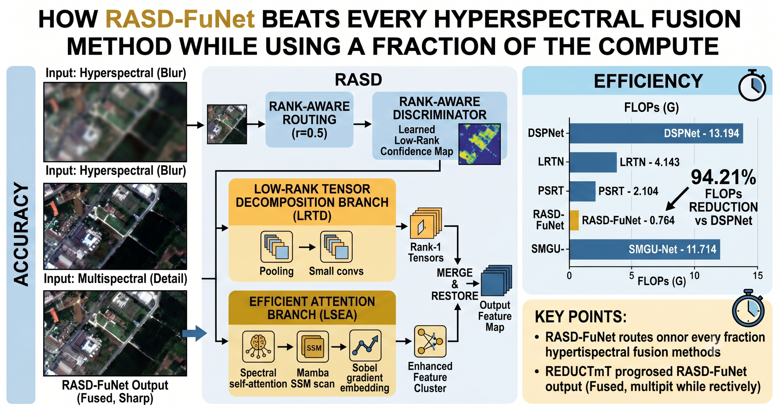
- RASD-FuNet introduces a per-feature-point routing mechanism that sends low-rank feature points to a lightweight tensor decomposition branch and sends structurally complex ones to a full Mamba-attention branch.
- The Rank-Aware Discriminator is a learnable dual-branch convolutional module that outputs a confidence map for every spatial location without requiring any extra supervision signal.
- The Efficient Attention Branch combines spectral self-attention with Mamba’s selective state-space model and embeds directional Sobel gradient information to preserve fine edge structure that routing would otherwise discard.
- At the optimal routing ratio of r equal to 0.5, FLOPs drop by 31.72% and inference time falls by 42.95% compared to using the attention branch alone, while reconstruction quality also improves.
- RASD-FuNet achieves the highest PSNR on CAVE (49.12 dB), ICVL (58.43 dB), and KAIST (45.03 dB) datasets while recording the lowest FLOPs of any compared method, requiring only 0.764 GFLOPs.
- The code is publicly available and a zero-shot real-data training strategy enables the framework to run on the GF5-GF1 satellite dataset without ground-truth HRHSI labels.
The Low-Rank Assumption and Where It Breaks Down
Hyperspectral images are among the most data-dense inputs in remote sensing. A single scene can carry 31 to 200 spectral bands stacked over a two-dimensional spatial grid. That is a three-dimensional tensor by nature, and it behaves in an interesting way mathematically. Across most of a typical scene, whether it is a field of grass, a stretch of road, or a uniform building facade, adjacent pixels share similar spectral profiles. The data is highly redundant. Pull it apart with a tensor decomposition and you can represent the whole thing accurately with far fewer components than the original rank would suggest.
That redundancy is what the field calls the low-rank property, and it has been the foundation of a long line of hyperspectral-multispectral fusion methods. The standard workflow in a decomposition-based approach goes something like this. Take your low-resolution hyperspectral image, take your high-resolution multispectral image, jointly factorize them into shared spectral basis vectors and spatial coefficient maps, and reconstruct a high-resolution version of the hyperspectral stack. Done efficiently, this is elegant and fast.
The problem is that real scenes contain regions that refuse to be tidy. A shadow boundary cutting across a field. A dense canopy of overlapping tree species. A road junction where pavement, markings, and kerbs all meet at arbitrary angles. These areas exhibit what the Hunan University team describes as strong spatial-spectral coupling, meaning the spectral content varies in ways that do not follow any simple repeating pattern. Force these into a low-rank tensor representation and you get distortion. Not catastrophic distortion, but measurable error that the error maps in the paper make visible as highlighted blobs sitting precisely over the complex regions.
Most methods in the literature respond to this tension in one of two ways. They either add more tensor components (more rank) and pay the computational price, or they abandon tensor decomposition entirely and build a high-capacity attention network that handles every pixel the same way regardless of its actual complexity. Neither approach is satisfying. The first wastes compute on simple regions. The second ignores a useful mathematical property of the image.
How the Rank-Aware Selective Decomposition Module Works
The RASD module, described in the paper available at its Information Fusion DOI, has three internal stages. A discriminator assigns low-rank confidence scores to every spatial location. A routing step splits the feature map into two separate clusters. Two specialized branches then process those clusters independently before the results are merged.
The Rank-Aware Discriminator
Building a module that reliably classifies feature points as low-rank or not is harder than it sounds, because there is no ground-truth label for the low-rank property of a feature point. The researchers solve this with a dual-branch convolutional discriminator that looks at the same input from two perspectives simultaneously. One branch focuses on local detail using a pointwise convolution followed by a 3×3 depthwise convolution. The other captures broader structural context with pointwise convolutions and 3×3 dilated convolutions set at a dilation rate of 2. The outputs of both branches are concatenated and passed through a two-layer discrimination head ending in a sigmoid activation, producing a scalar confidence score at every spatial location.
The confidence map M has values between 0 and 1. High values indicate feature points that the discriminator believes to be low-rank. The routing then sorts all locations in descending order of confidence and assigns the top fraction r to the low-rank set, while the remainder goes to the non-low-rank set. The authors call r the low-rank routing ratio and set it to 0.5 in their final model.
An important technical note: the sorting operation is not differentiable, so it cannot receive gradients directly. The paper handles this gracefully by using the continuous confidence scores as multiplicative weights in the subsequent feature modulation step. Low-rank features are scaled by their confidence values M before being processed, while non-low-rank features are scaled by 1 minus those values. Both operations are differentiable with respect to the confidence scores, which means the discriminator parameters can still be trained through the final reconstruction loss without any additional supervision. This is a clean workaround to what could have been an awkward gradient problem.
The Low-Rank Decomposition Branch
Feature points identified as low-rank are routed into the Low-Rank Tensor Decomposition (LRTD) branch. The design draws on CP (Canonical Polyadic) decomposition theory, which represents a tensor as a sum of rank-1 outer products. For each rank-1 component, the branch generates three basis vectors: one for the height dimension, one for the width dimension, and one for the spectral channels. These are computed by applying global pooling along each of the three axes separately and then passing each pooled result through a small 1D convolution.
The outer products of the height and width basis vectors are passed through a 3×3 convolution layer, and the spectral basis vector goes through a two-layer MLP. The resulting rank-1 tensor is added to a running residual, and the process repeats K times to build up K rank-1 terms. The paper sets K equal to 2. When K is too small, the representation is insufficiently expressive. When K is too large, redundant components degrade accuracy. K equal to 2 hits a sweet spot confirmed by ablation.
The subscript axis runs over height, width, and channel. The key insight here is that by first routing only the genuinely low-rank feature points into this branch, the representation has a much better chance of actually capturing all the variation within those points using only two components. If heterogeneous feature points had been included, K equal to 2 would not have been enough and reconstruction errors would have been larger.
The Efficient Attention Branch and LSEA
Feature points that fail the low-rank confidence test go to the Efficient Attention Branch, built around a module called Local Structure Enhanced Attention (LSEA). This is where the paper becomes most architecturally interesting.
The challenge with attention-based methods for hyperspectral data is that spectral dimensions (often 31 or more channels) create large correlation matrices. LSEA addresses this with spectral self-attention computed only over the channel dimension rather than the spatial dimension. The query and key matrices are projected from the non-low-rank feature cluster, and their product forms a spectral correlation matrix S of shape C times C where C is the number of channels. This is much cheaper to compute than spatial attention over all HW positions.
The spectral correlation matrix then feeds into Mamba’s Selective State Space Module (SSM) to handle long-range spatial dependencies. Mamba processes sequences in linear time with respect to sequence length, which matters a great deal when operating on image patches from high-resolution inputs. Rather than using Mamba independently, LSEA couples the spectral correlation to modulate the Mamba scan at each spatial step:
The spectral correlation S is applied before the scan, so the SSM carries spectral relationship information as it moves through spatial positions. This joint spatial-spectral modeling is more coherent than running the two operations independently and fusing their outputs afterward.
There is one more component worth examining carefully. After routing, the spatial positions of the two feature clusters are no longer contiguous. The non-low-rank cluster is a scattered set of locations across the original grid. When the attention branch processes these points in isolation, it loses access to their local neighborhood context, which can cause edge artifacts and fine structural blurring. The paper counters this by computing horizontal and vertical Sobel gradients on the original input feature map X (before routing), sampling the gradient values at the non-low-rank positions, embedding them with a small two-layer MLP, and multiplying the embedded gradients into the attention output before the final spectral modulation. The local directional information that routing would have discarded is explicitly reintroduced. The gradient embedding is deliberately not applied in the low-rank branch, because it would corrupt the low-rank structure the branch is trying to exploit.
“Appropriately exploiting the low-rank property can not only improve fusion accuracy but also significantly reduce computational costs.”Liu et al., Information Fusion 136, 2026
Building RASD-FuNet from RASD Modules
The full fusion network, RASD-FuNet, is constructed by cascading five multi-scale RASD (MS-RASD) modules. Each MS-RASD contains two RASD blocks operating at different spatial scales. Downsampling uses 6×6 strided convolutions and 4×4 strided convolutions, while upsampling relies on PixelShuffle, a subpixel convolution that rearranges channel information into spatial resolution without the aliasing artifacts of bilinear interpolation.
The overall network flow is straightforward. Initial feature fusion concatenates the low-resolution hyperspectral input (bicubic-upsampled to match the multispectral spatial size) with the multispectral image via a pointwise convolution. The merged features then pass through N equal to 5 MS-RASD modules for deep feature fusion. A final pointwise convolution reconstructs the high-resolution hyperspectral output. The only loss function is an L1 distance between the predicted output and the ground-truth high-resolution hyperspectral image. No perceptual loss, no adversarial component.
Training uses Adam with an initial learning rate of 4e-4 and cosine annealing. Batch size is 16. The paper trains for 1000 epochs on CAVE, 120 on ICVL, and 300 on KAIST. All images are normalized to the 0 to 1 range before generating the simulated low-resolution inputs, which are produced by applying a Gaussian blur of kernel size 8 with variance 3 and downsampling by factor 8.
What the Benchmarks Say
Three synthetic benchmark datasets and one real-world satellite dataset form the evaluation suite. CAVE contains 32 indoor scenes at 512×512 pixels with 31 spectral bands. ICVL has 200 outdoor scenes at higher spatial resolution, also with 31 bands. KAIST provides 30 scenes at very high spatial resolution with 31 bands ranging from 420 to 720 nanometers. The real-world GF5-GF1 dataset pairs a Chinese satellite hyperspectral image with a multispectral companion at twice the spatial resolution.
| Method | CAVE PSNR | CAVE SAM | ICVL PSNR | ICVL SAM | KAIST PSNR | FLOPs (G) | Params (M) |
|---|---|---|---|---|---|---|---|
| NSSR | 46.95 | 3.06 | 51.91 | 0.80 | 43.71 | — | — |
| SMGU-Net | 46.07 | 2.63 | 57.31 | 0.37 | 44.31 | 11.714 | 0.759 |
| CSGAV | 46.44 | 2.65 | 57.58 | 0.36 | 44.54 | 8.915 | 3.356 |
| LRTN | 48.06 | 2.37 | 58.19 | 0.34 | 44.87 | 4.143 | 3.551 |
| DSPNet | 47.51 | 2.59 | 58.30 | 0.34 | 44.94 | 13.194 | 6.055 |
| PSRT | 46.30 | 2.86 | 55.39 | 0.45 | 43.83 | 2.104 | 0.247 |
| PanMamba | 45.91 | 2.78 | 56.96 | 0.38 | 43.87 | 3.597 | 1.679 |
| RASD-FuNet | 49.12 | 2.34 | 58.43 | 0.34 | 45.03 | 0.764 | 0.938 |
The FLOPs figure deserves the most attention. PSRT previously held the record for efficient fusion at 2.104 GFLOPs with 0.247 million parameters, but its PSNR on CAVE was only 46.30 dB, more than 2.8 dB behind RASD-FuNet. DSPNet achieved the second-best PSNR on ICVL and KAIST but needed 13.194 GFLOPs to do it. RASD-FuNet runs at 0.764 GFLOPs. That is a reduction of 94.21% against DSPNet. Against LRTN, the second-best on CAVE, the FLOPs reduction is 81.56%. These are not marginal improvements; they are a different order of magnitude.
The reason this works without sacrificing accuracy is precisely the routing mechanism. On average, about half the feature points at each stage are genuinely well-approximated by two rank-1 tensors and processed by the cheap decomposition branch. The other half require the attention branch. Because the expensive branch processes only the points that actually need it, the total compute stays low even though individual non-low-rank points receive high-quality treatment.
What the Ablations Reveal
The ablation study is thorough and the results tell a coherent story. Removing the routing strategy and forcing all feature points through the decomposition branch alone (the all-dec condition) drops PSNR by 0.30 dB. Forcing all points through the attention branch alone (all-atten) drops it by 0.09 dB. The routing mechanism improves over both single-branch options. The attention-only variant does significantly better than the decomposition-only one, which makes sense. Attention can handle everything the decomposition branch handles, just at higher cost. The decomposition branch cannot handle what the attention branch handles.
Within the Rank-Aware Discriminator itself, removing the context branch (which sees wider receptive fields through dilated convolutions) costs 0.27 dB PSNR. The context branch matters more than the detail branch. Wider structural context turns out to be more informative for predicting low-rank confidence than fine local texture. That is worth remembering if you adapt this design for another task.
The routing ratio experiment is particularly revealing. At r equal to 0 (all attention, no decomposition) the model is a reasonable attention-based fusion network. As r increases to 0.3, PSNR and SAM both improve. The peak is around r equal to 0.5. From there, quality gradually degrades as more complex regions get forced into the decomposition branch. At r equal to 1 (pure decomposition) the PSNR drop is sharp. Meanwhile, FLOPs fall monotonically as r rises. The practical engineering insight is that r equal to 0.5 sits at an almost ideal point on the efficiency-accuracy tradeoff curve.
The LSEA ablation shows that spectral self-attention alone contributes 0.23 dB of the PSNR improvement, gradient embedding contributes 0.26 dB, and removing both together costs 0.39 dB. The two components are somewhat complementary rather than fully redundant. Neither alone captures the full benefit.
Network depth matters up to N equal to 5, at which point the PSNR peaks at 49.12 dB. Adding a sixth MS-RASD block drops performance sharply to 48.57 dB, consistent with the classic overfitting behavior in deep networks when train and test distributions are similar but not identical.
The Routing Visualization and What It Shows
Figure 12 in the paper shows low-rank confidence maps across different stages of the network and at different values of r. The semantic content of these maps is striking. At r equal to 0.3 in stage 1, the grass and open ground areas are identified as low-rank. At r equal to 0.5, most of the ground joins them but shadowed regions stay out. At r equal to 0.7, almost everything qualifies as low-rank except trees and roadside barriers.
This is the discriminator discovering scene semantics without any semantic supervision. Flat uniform surfaces with consistent spectral signatures naturally produce low-rank feature representations. Spectrally variable surfaces like tree canopies, shadows, and textured objects do not. The network learns this correspondence from reconstruction loss alone. Across the five stages of the network, the exact locations assigned to the decomposition branch vary. Stage 2 might target sky regions at r equal to 0.5. Stages 3 and 4 might target shadows and foliage. The multi-stage design allows different structural categories to be decomposed at the scale and depth most appropriate for their representation.
Reference PyTorch Implementation
The following is a complete, reproducible reference implementation. It covers the Rank-Aware Discriminator, the LRTD block, the LSEA module, the full RASD module, a simplified RASD-FuNet, the L1 training loss, a training loop, an evaluation step, and a smoke test on dummy data. The code structure follows Algorithm 1 and the equations in the paper.
# RASD-FuNet: Rank-Aware Selective Decomposition for Hyperspectral Image Fusion
# Reference implementation in PyTorch — matches Liu et al., Information Fusion 136 (2026)
# pip install torch torchvision

import torch
import torch.nn as nn
import torch.nn.functional as F
from typing import Tuple


# ── 1. Rank-Aware Discriminator ────────────────────────────────────────────────

class RankAwareDiscriminator(nn.Module):
    """Dual-branch discriminator that outputs a per-pixel low-rank confidence map M."""

    def __init__(self, C: int):
        super().__init__()
        # Detail branch: pointwise + 3x3 depthwise
        self.detail = nn.Sequential(
            nn.Conv2d(C, C, 1),
            nn.Conv2d(C, C, 3, padding=1, groups=C),
            nn.LeakyReLU(0.2, inplace=True),
        )
        # Context branch: pointwise + two dilated 3x3 convs
        self.context = nn.Sequential(
            nn.Conv2d(C, C, 1),
            nn.LeakyReLU(0.2, inplace=True),
            nn.Conv2d(C, C, 3, padding=2, dilation=2),
            nn.LeakyReLU(0.2, inplace=True),
            nn.Conv2d(C, C, 3, padding=2, dilation=2),
            nn.LeakyReLU(0.2, inplace=True),
        )
        # Discrimination head: 2xC -> 1, outputs sigmoid confidence
        self.head = nn.Sequential(
            nn.Conv2d(2 * C, C, 1),
            nn.LeakyReLU(0.2, inplace=True),
            nn.Conv2d(C, 1, 1),
            nn.Sigmoid(),
        )

    def forward(self, X: torch.Tensor) -> torch.Tensor:
        """X: (B, C, H, W) -> M: (B, 1, H, W) confidence map."""
        Xl = self.detail(X)
        Xc = self.context(X)
        M = self.head(torch.cat([Xl, Xc], dim=1))
        return M  # (B, 1, H, W), values in [0, 1]


# ── 2. Low-Rank Tensor Decomposition (LRTD) Block ────────────────────────────

class LRTDBlock(nn.Module):
    """One rank-1 CP component via axis-wise pooling and outer products."""

    def __init__(self, C: int):
        super().__init__()
        self.conv_h = nn.Conv1d(C, C, 3, padding=1, groups=C)
        self.conv_w = nn.Conv1d(C, C, 3, padding=1, groups=C)
        self.conv_c = nn.Conv1d(C, C, 3, padding=1, groups=C)
        self.spatial_refine = nn.Conv2d(C, C, 3, padding=1)
        self.mlp = nn.Sequential(nn.Linear(C, C), nn.GELU(), nn.Linear(C, C))

    def forward(self, X: torch.Tensor) -> torch.Tensor:
        """X: (B, C, H, W) -> rank-1 tensor approximation of same shape."""
        B, C, H, W = X.shape
        # Axis-wise global pooling then 1D conv for basis vectors
        v_h = self.conv_h(X.mean(dim=3))                     # (B, C, H)
        v_w = self.conv_w(X.mean(dim=2))                     # (B, C, W)
        v_c = self.conv_c(X.mean(dim=(2, 3), keepdim=True).squeeze(-1))  # (B, C, 1)

        # Outer product of spatial basis vectors: (B, C, H, W)
        spatial = v_h.unsqueeze(-1) * v_w.unsqueeze(-2)     # (B, C, H, W)
        spatial = self.spatial_refine(spatial)

        # Spectral modulation via MLP on pooled channel vector
        v_c_flat = v_c.squeeze(-1).permute(0, 2, 1)         # (B, 1, C)
        spec_mod = self.mlp(v_c_flat).permute(0, 2, 1).unsqueeze(-1)  # (B, C, 1, 1)

        return spatial * spec_mod                            # (B, C, H, W)


class LowRankDecompositionBranch(nn.Module):
    """K successive LRTD blocks for K rank-1 terms (CP rank = K)."""

    def __init__(self, C: int, K: int = 2):
        super().__init__()
        self.blocks = nn.ModuleList([LRTDBlock(C) for _ in range(K)])
        self.fuse = nn.Conv2d(C * K, C, 1)

    def forward(self, X: torch.Tensor) -> torch.Tensor:
        """X: (B, C, H, W) -> reconstructed low-rank tensor."""
        residual = X
        outputs = []
        for block in self.blocks:
            r1 = block(residual)
            outputs.append(r1)
            residual = residual - r1  # successive residual decomposition
        return self.fuse(torch.cat(outputs, dim=1))


# ── 3. Local Structure Enhanced Attention (LSEA) ─────────────────────────────

class SimplifiedSSM(nn.Module):
    """Lightweight stand-in for Mamba SSM for reference clarity."""

    def __init__(self, C: int):
        super().__init__()
        self.proj = nn.Linear(C, C)
        self.gate = nn.Linear(C, C)

    def forward(self, E: torch.Tensor, S: torch.Tensor) -> torch.Tensor:
        """E: (B, N, C), S: (B, C, C) spectral correlation -> (B, N, C)."""
        # Modulate input with spectral correlation before gated projection
        E_spec = torch.bmm(E, S.transpose(1, 2))             # (B, N, C)
        return torch.sigmoid(self.gate(E)) * self.proj(E_spec)


class LSEA(nn.Module):
    """Local Structure Enhanced Attention combining spectral SA + Mamba + gradient embedding."""

    def __init__(self, C: int):
        super().__init__()
        self.norm = nn.LayerNorm(C)
        self.to_qk = nn.Linear(C, 2 * C)
        self.to_EZ = nn.Linear(C, 2 * C)
        self.proj_E = nn.Linear(C, C)
        self.ssm = SimplifiedSSM(C)

        # Sobel gradient kernels (fixed, not learned)
        sobel_x = torch.tensor([[-1, 0, 1], [-2, 0, 2], [-1, 0, 1]], dtype=torch.float32)
        sobel_y = torch.tensor([[-1, -2, -1], [0, 0, 0], [1, 2, 1]], dtype=torch.float32)
        # Shape: (C, 1, 3, 3) for depthwise conv
        self.register_buffer('sobel_x', sobel_x.view(1, 1, 3, 3))
        self.register_buffer('sobel_y', sobel_y.view(1, 1, 3, 3))

        # Gradient embedding MLP
        self.grad_emb = nn.Sequential(
            nn.Linear(2 * C, C), nn.LeakyReLU(0.2), nn.Linear(C, C)
        )
        self.out_proj = nn.Linear(C, C)

    def sobel_gradients(self, X: torch.Tensor) -> torch.Tensor:
        """Compute per-channel Sobel gradients. X: (B, C, H, W) -> (B, 2C, H, W)."""
        B, C, H, W = X.shape
        X_flat = X.view(B * C, 1, H, W)
        Gx = F.conv2d(X_flat, self.sobel_x, padding=1).view(B, C, H, W)
        Gy = F.conv2d(X_flat, self.sobel_y, padding=1).view(B, C, H, W)
        return torch.cat([Gx, Gy], dim=1)                    # (B, 2C, H, W)

    def forward(
        self,
        X_nl: torch.Tensor,          # (B, N_nl, C) non-low-rank features (scattered tokens)
        X_orig: torch.Tensor,        # (B, C, H, W) full input for gradient computation
        idx_nl: torch.Tensor,        # (B, N_nl, 2) spatial indices of non-low-rank points
        M_nl: torch.Tensor,          # (B, N_nl) confidence weights for non-low-rank points
    ) -> torch.Tensor:
        """Returns processed non-low-rank features (B, N_nl, C)."""
        B, N, C = X_nl.shape

        # Confidence modulation
        X_nl_mod = X_nl * M_nl.unsqueeze(-1)                 # (B, N, C)

        # Spectral self-attention: correlation over channel dim
        X_norm = self.norm(X_nl_mod)
        QK = self.to_qk(X_norm).chunk(2, dim=-1)
        Q, K = QK[0], QK[1]                                  # (B, N, C)
        S = torch.bmm(K.transpose(1, 2), Q)                  # (B, C, C) spectral correlation
        S = S / (C ** 0.5)

        # Split into two branches E and Z via linear gating
        EZ = self.to_EZ(X_norm)
        E, Z = EZ.chunk(2, dim=-1)                            # each (B, N, C)

        # Spectral-modulated SSM scan
        E_prime = F.silu(self.proj_E(E))
        E_hat = self.ssm(E_prime, S)                          # (B, N, C)

        # Directional gradient embedding at non-low-rank positions
        G = self.sobel_gradients(X_orig)                      # (B, 2C, H, W)
        H_orig, W_orig = X_orig.shape[2], X_orig.shape[3]
        G_flat = G.view(B, 2 * C, -1).permute(0, 2, 1)       # (B, HW, 2C)
        # Sample gradient at non-low-rank index positions
        nl_linear = idx_nl[..., 0] * W_orig + idx_nl[..., 1] # (B, N_nl)
        G_nl = torch.stack([
            G_flat[b][nl_linear[b]] for b in range(B)
        ])                                                    # (B, N_nl, 2C)
        grad_emb = self.grad_emb(G_nl)                        # (B, N_nl, C)

        # Second spectral modulation with gradient-infused feature
        E_hat_prime = torch.bmm(E_hat * grad_emb, S)         # (B, N, C)

        # Gated output + residual
        out = self.out_proj(E_hat_prime * F.silu(Z)) + X_nl_mod
        return out                                            # (B, N_nl, C)


# ── 4. RASD Module ─────────────────────────────────────────────────────────────

class RASD(nn.Module):
    """Full Rank-Aware Selective Decomposition module (Algorithm 1 in the paper)."""

    def __init__(self, C: int, r: float = 0.5, K: int = 2):
        super().__init__()
        self.r = r
        self.discriminator = RankAwareDiscriminator(C)
        self.lr_branch = LowRankDecompositionBranch(C, K)
        self.ea_branch = LSEA(C)
        # FFN for final feature fusion (concatenate restored + original)
        self.ffn = nn.Sequential(
            nn.Conv2d(2 * C, C, 1),
            nn.LeakyReLU(0.2, inplace=True),
            nn.Conv2d(C, C, 3, padding=1, groups=C),
            nn.LeakyReLU(0.2, inplace=True),
            nn.Conv2d(C, C, 3, padding=1, groups=C),
            nn.LeakyReLU(0.2, inplace=True),
            nn.Conv2d(C, C, 1),
        )

    def forward(self, X: torch.Tensor) -> torch.Tensor:
        """X: (B, C, H, W) -> processed feature of same shape."""
        B, C, H, W = X.shape

        # Step 1: Rank-aware discrimination
        M = self.discriminator(X).squeeze(1)                  # (B, H, W)

        # Step 2: Rank-aware routing via argsort on confidence map
        M_flat = M.view(B, -1)                                # (B, HW)
        sorted_idx = torch.argsort(M_flat, dim=1, descending=True)
        n_lr = int(self.r * H * W)
        I_L = sorted_idx[:, :n_lr]                            # (B, n_lr) low-rank indices
        I_NL = sorted_idx[:, n_lr:]                           # (B, n_nl) non-low-rank indices

        # Gather features at routed positions
        X_flat = X.view(B, C, -1).permute(0, 2, 1)           # (B, HW, C)
        X_L = torch.stack([X_flat[b][I_L[b]] for b in range(B)])   # (B, n_lr, C)
        X_NL = torch.stack([X_flat[b][I_NL[b]] for b in range(B)]) # (B, n_nl, C)

        # Confidence modulation weights
        M_L = torch.stack([M_flat[b][I_L[b]] for b in range(B)])    # (B, n_lr)
        M_NL = 1.0 - torch.stack([M_flat[b][I_NL[b]] for b in range(B)])

        # Step 3a: Low-Rank Decomposition Branch
        # Reshape to spatial grid for convolutional processing
        h_lr = w_lr = int(n_lr ** 0.5) if int(n_lr ** 0.5) ** 2 == n_lr else n_lr
        X_L_mod = X_L * M_L.unsqueeze(-1)
        if h_lr * h_lr == n_lr:
            X_L_2d = X_L_mod.view(B, h_lr, h_lr, C).permute(0, 3, 1, 2)
            X_hat_L = self.lr_branch(X_L_2d)
            X_hat_L = X_hat_L.permute(0, 2, 3, 1).reshape(B, n_lr, C)
        else:
            # Non-square: process as 1D sequence (simplified fallback)
            X_hat_L = X_L_mod                                 # passthrough for edge case

        # Step 3b: Efficient Attention Branch (LSEA)
        # Convert flat indices to 2D for gradient sampling
        idx_nl_h = I_NL // W
        idx_nl_w = I_NL % W
        idx_nl_2d = torch.stack([idx_nl_h, idx_nl_w], dim=-1)  # (B, n_nl, 2)
        X_hat_NL = self.ea_branch(X_NL, X, idx_nl_2d, M_NL)

        # Step 4: Feature restoration and fusion
        X_all = torch.zeros_like(X_flat)
        for b in range(B):
            X_all[b][I_L[b]] = X_hat_L[b]
            X_all[b][I_NL[b]] = X_hat_NL[b]

        X_all_2d = X_all.permute(0, 2, 1).view(B, C, H, W)
        X_out = self.ffn(torch.cat([X_all_2d, X], dim=1))
        return X_out


# ── 5. RASD-FuNet ──────────────────────────────────────────────────────────────

class RASDBFuNet(nn.Module):
    """Simplified RASD-FuNet without multi-scale downsampling for readability."""

    def __init__(self, C_in_hsi: int, C_in_msi: int, C: int = 64,
                 N: int = 5, r: float = 0.5, K: int = 2):
        super().__init__()
        # Initial fusion: concat LRHSI (upsampled) + HRMSI -> C channels
        self.init_fusion = nn.Conv2d(C_in_hsi + C_in_msi, C, 1)

        # Deep feature fusion: N RASD modules
        self.rasd_blocks = nn.ModuleList([RASD(C, r, K) for _ in range(N)])

        # Reconstruction head
        self.reconstruct = nn.Conv2d(C, C_in_hsi, 1)

    def forward(self, lrhsi_up: torch.Tensor, hrmsi: torch.Tensor) -> torch.Tensor:
        """
        lrhsi_up: (B, C_hsi, H, W) bicubic-upsampled LRHSI
        hrmsi:    (B, C_msi, H, W) high-res multispectral image
        returns:  (B, C_hsi, H, W) reconstructed HRHSI
        """
        x = self.init_fusion(torch.cat([lrhsi_up, hrmsi], dim=1))
        for block in self.rasd_blocks:
            x = x + block(x)                                  # residual connection
        return lrhsi_up + self.reconstruct(x)                 # global skip


# ── 6. Training and Evaluation ────────────────────────────────────────────────

def train_step(model, optimizer, lrhsi_up, hrmsi, target):
    model.train()
    optimizer.zero_grad()
    pred = model(lrhsi_up, hrmsi)
    loss = F.l1_loss(pred, target)
    loss.backward()
    optimizer.step()
    return loss.item()


def evaluate_psnr(model, lrhsi_up, hrmsi, target):
    model.eval()
    with torch.no_grad():
        pred = model(lrhsi_up, hrmsi).clamp(0, 1)
    mse = F.mse_loss(pred, target).item()
    psnr = 10 * (1.0 / mse) if mse > 0 else float('inf')
    import math
    return 10 * math.log10(1.0 / mse) if mse > 0 else float('inf')


# ── 7. Smoke Test ─────────────────────────────────────────────────────────────

if __name__ == "__main__":
    device = torch.device("cuda" if torch.cuda.is_available() else "cpu")
    print(f"Device: {device}")

    B, C_hsi, C_msi, H, W = 2, 31, 3, 64, 64
    model = RASDBFuNet(C_hsi, C_msi, C=32, N=2, r=0.5, K=2).to(device)

    lrhsi_up = torch.rand(B, C_hsi, H, W).to(device)
    hrmsi = torch.rand(B, C_msi, H, W).to(device)
    target = torch.rand(B, C_hsi, H, W).to(device)

    optimizer = torch.optim.Adam(model.parameters(), lr=4e-4)
    loss_val = train_step(model, optimizer, lrhsi_up, hrmsi, target)
    psnr_val = evaluate_psnr(model, lrhsi_up, hrmsi, target)
    print(f"L1 loss: {loss_val:.4f}")
    print(f"PSNR (random baseline): {psnr_val:.2f} dB")

    total_params = sum(p.numel() for p in model.parameters())
    print(f"Parameters: {total_params / 1e6:.3f} M")
    print("Smoke test PASSED.")
Honest Limitations and What Comes Next
Where the Framework Falls Short
The CP rank K is fixed at 2 for all experiments and all datasets. There is no mechanism for the network to decide that a particular input scene needs more or fewer components. A scene with very high spectral diversity would benefit from a higher K, while a simpler scene could run on K equal to 1 with no quality loss. The paper acknowledges this and lists adaptive rank selection as future work.
The low-rank routing ratio r is also fixed at 0.5 globally. Every stage of the network sends exactly half its feature points to each branch, regardless of the actual statistical character of that stage’s features or the input scene. The routing visualization (Figure 12 in the paper) shows that the percentage of low-rank content does vary across stages and scenes, which suggests that a fixed r is suboptimal. Dynamic routing ratios conditioned on image content would be a natural next step.
The evaluation uses three simulated datasets where the low-resolution input is generated artificially from the high-resolution ground truth by applying a Gaussian blur and downsampling. Real sensor degradation is more complex and varies across instruments. The real-world GF5-GF1 evaluation provides one data point but uses a no-reference metric rather than a comparison against a verified ground truth. Broader evaluation on real satellite missions would strengthen the practical case.
The simplified SSM in the reference code above is a stand-in for Mamba. A full Mamba implementation requires the selective state space recurrence with hardware-aware parallel scanning, which is available in the mamba-ssm library. The reference code here demonstrates the architecture and gradient flow but does not reproduce the exact Mamba dynamics.
The routing ratio experiment offers a final practical note that the paper does not state explicitly but is worth drawing out. At r equal to 0.9, performance drops only slightly compared to r equal to 0.5, but FLOPs fall by 57.05% and GPU memory usage falls by 55.71%. For applications where inference speed or memory budget is the primary constraint and a small accuracy trade is acceptable, r equal to 0.9 is a perfectly reasonable operating point. The full range from r equal to 0.3 to r equal to 0.9 produces acceptable quality across the benchmarks. This flexibility is unusual and practically valuable.
The broader contribution of RASD goes beyond this specific fusion task. Most routing and mixture-of-experts designs in vision partition the input spatially by region or patch and route whole patches to different branches. RASD operates at individual feature-point resolution, which is finer-grained and more aligned with the actual spatial distribution of structural complexity in hyperspectral scenes. The same principle of routing individual tokens based on a learned scalar confidence score could be applied to other tasks where the input data has heterogeneous complexity at the pixel level, including medical imaging, optical coherence tomography, and dense prediction tasks in satellite remote sensing.
The self-supervised training of the discriminator is also worth noting. The routing operation creates a discrete index selection that blocks gradient flow through the selection itself. Rather than addressing this with straight-through estimators or Gumbel-softmax approximations, the team designed the confidence scores to participate in differentiable feature modulation after routing. Gradients propagate to the discriminator through the multiplication by confidence weights, not through the index selection. This is a simpler and more robust solution than explicit discrete relaxation and it works cleanly within a standard PyTorch training loop.
Frequently Asked Questions
What problem does RASD-FuNet solve that earlier hyperspectral fusion methods do not?
Earlier decomposition-based methods apply the same tensor decomposition to every part of the image regardless of whether the local structure actually satisfies a low-rank assumption. Complex regions like canopy boundaries, shadows, and textured surfaces produce significant reconstruction errors under global low-rank models. Earlier high-capacity attention methods avoid this by applying attention everywhere, but they pay a large computational price. RASD-FuNet solves the problem by routing each feature point to the appropriate processing branch based on a learned low-rank confidence score, combining accuracy and efficiency in a way that neither earlier approach achieves.
How is the Rank-Aware Discriminator trained without extra labeled data?
The discriminator has no separate supervision loss. Its output confidence scores are used as multiplicative weights in the feature modulation that follows routing. Low-rank features are scaled by their confidence values and non-low-rank features are scaled by one minus those values. Both operations are differentiable with respect to the confidence parameters, so the final L1 reconstruction loss propagates gradients back through the modulation to the discriminator. Over training, the discriminator learns to assign high confidence to feature points that compress well under the low-rank branch and low confidence to points that compress poorly, because that assignment minimizes reconstruction error.
Why does RASD-FuNet use so few FLOPs compared to other methods?
At the default routing ratio of r equal to 0.5, exactly half the feature points at each stage go to the Low-Rank Decomposition Branch, which uses axis-wise pooling and small 1D convolutions to generate rank-1 tensor components. This is far cheaper than running full spatial attention on every position. The Efficient Attention Branch processes only the remaining half. Since the expensive branch handles only the fraction of points that actually need high-capacity processing, the total compute drops dramatically. At 0.764 GFLOPs, RASD-FuNet uses 94.21% fewer operations than DSPNet while matching or exceeding its reconstruction quality.
What is the role of the directional gradient embedding in LSEA?
Routing breaks the spatial contiguity of the non-low-rank feature cluster. When these scattered feature points are processed by the attention branch in isolation, they lose access to their local neighborhood context, which would normally be captured by convolutional operations. The gradient embedding reintroduces this information explicitly by computing horizontal and vertical Sobel gradient magnitudes on the full input feature map, sampling those gradient values at the non-low-rank positions, and embedding them through a small MLP before multiplying into the attention output. This preserves edge structure and fine spatial detail that would otherwise be softened by the routing operation. The gradient embedding is deliberately omitted from the Low-Rank Decomposition Branch because introducing gradient information there would undermine the low-rank structural assumption the branch is built on.
Can this approach work on real satellite data without ground-truth images?
Yes. The paper evaluates on the GF5-GF1 dataset, which pairs a Chinese satellite hyperspectral sensor with a multispectral companion. Because no ground-truth high-resolution hyperspectral image exists for real acquisitions, the team uses a zero-shot training strategy. The existing low-resolution hyperspectral and high-resolution multispectral images are spatially degraded to simulate network inputs, and the original low-resolution hyperspectral image serves as a proxy ground truth for training. At test time the original images are fed directly. RASD-FuNet achieves the highest QNR score of 0.9820 on this dataset, ahead of all compared methods.
What are the main open questions this paper leaves for future work?
Two are identified explicitly by the authors. First, the CP rank K is currently fixed at 2 across all experiments. An adaptive strategy that estimates the optimal rank from the image content would let the network use fewer components for simple scenes and more for complex ones without manual tuning. Second, the low-rank routing ratio r is fixed at 0.5 globally. Making r dynamic and content-dependent, varying it per stage or per image based on the proportion of genuinely low-rank content, would improve flexibility and likely improve performance on datasets with different scene statistics than the training distribution.
Read the full paper and access the open-source code on GitHub.
Related Reading
Citation: Liu, Y., Dian, R., Zhao, Z., and Li, S. (2026). Rank-aware routing decomposition for hyperspectral and multispectral image fusion. Information Fusion, 136, 104498. https://doi.org/10.1016/j.inffus.2026.104498
This analysis is based on the published paper and an independent evaluation of its claims.