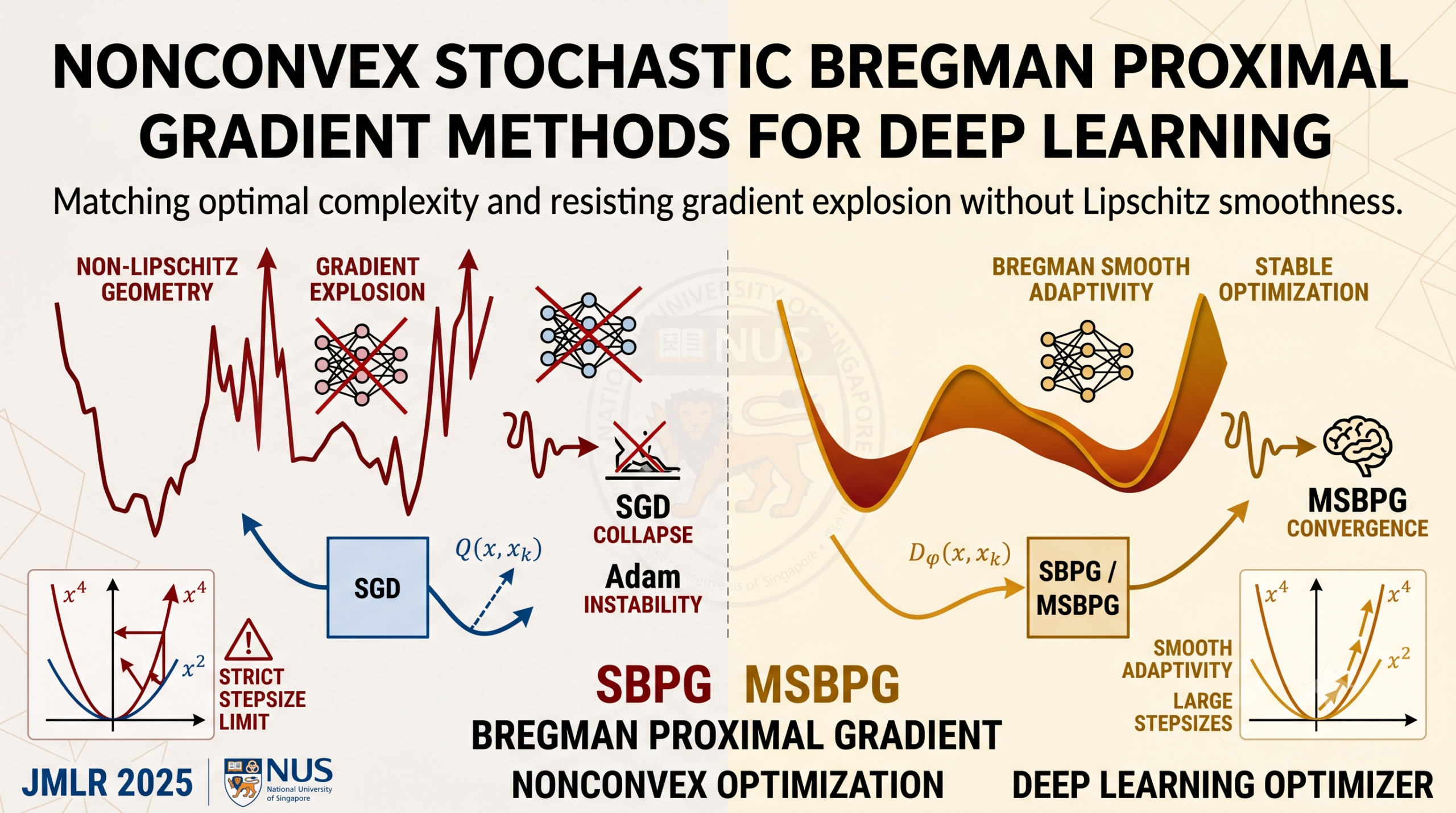
A team from the National University of Singapore built stochastic Bregman proximal gradient methods that drop the Lipschitz continuity requirement, match the optimal O(ε⁻⁴) sample complexity, and resist gradient explosion on architectures where standard optimizers collapse under large stepsizes or bad initialization.
- Standard SGD requires Lipschitz gradient continuity — a condition that fails for many real network loss functions, including simple polynomials like x⁴.
- SBPG replaces the quadratic SGD proximity term with a Bregman distance that adapts to the actual curvature of the objective via smooth adaptivity.
- The momentum variant MSBPG achieves the optimal O(ε⁻⁴) sample complexity with a mini-batch size of 1, removing the large batch requirement of vanilla SBPG.
- A polynomial kernel of degree r ≥ 4 gives MSBPG an automatic pull-back mechanism that scales down gradient steps when the parameter norm grows, resisting gradient explosion without clipping.
- Across VGG16, ResNet34, DenseNet121, LSTMs, and Transformer-XL, MSBPG matches or beats SGD and Adam on both accuracy and perplexity.
- The method tolerates stepsizes up to 5 and initialization scales up to 20 before failing — compared to roughly 0.6 and 4.6 for SGD on the same network.
The Problem With Quadratic Approximations
Every stochastic gradient method, at its heart, is solving the same local subproblem at each step. It builds a local model of the objective function, minimizes that model, and moves to the minimizer. The choice of model determines everything — the convergence rate, the stepsize sensitivity, the behavior when gradients explode.
Standard SGD uses a quadratic model. At the current point x^k, it approximates F(x) by a linear term plus a squared Euclidean penalty that keeps the next iterate close to the current one. The penalty’s weight is the reciprocal of the stepsize. The problem is that this quadratic model only provides a valid upper bound on F(x) when the gradient of F is Lipschitz continuous — meaning the curvature of F is bounded everywhere.
Take F(x) = x⁴. Its gradient is 4x³ and the Hessian is 12x². As x grows, the curvature grows without limit. No fixed quadratic model can upper-bound that function over an unbounded domain, and no fixed stepsize will keep the iterates stable. The practical consequence is familiar to anyone who has trained a deep network. Choose a stepsize that is too large and the loss spikes. Choose one that is too small and training crawls. The valid range is narrow, and finding it requires multiple runs with different hyperparameters.
Bregman proximal methods offer a different model. Instead of a squared Euclidean distance as the proximity term, they use a Bregman distance induced by a kernel function. The kernel can be chosen to match the curvature structure of the objective — and when it does, the resulting model provides a valid upper bound without any global Lipschitz constant. This property is called smooth adaptivity, and it is the conceptual foundation of the entire paper.
A function F is L-smooth adaptable with respect to kernel φ if Lφ plus F and Lφ minus F are both convex. For F(x) = x⁴, the kernel φ(x) = (1/2)x² + (1/4)x⁴ achieves smooth adaptivity with constant L = 4. The standard quadratic kernel requires a Lipschitz constant of 48 over the same domain. The Bregman model is geometrically closer to the true objective, which means the optimizer can take larger and more confident steps.
What SBPG Actually Does Differently
The core update rule for SBPG replaces the quadratic penalty in the SGD subproblem with a Bregman distance term. The subproblem at each iteration becomes minimizing the sum of the regularizer R(x), a linear term using the current stochastic gradient, and a scaled Bregman distance from the current point.
The Bregman distance D_φ(x, y) measures how much the kernel function φ at x exceeds its first-order approximation at y. When φ is the standard squared norm, this collapses exactly to the squared Euclidean distance and SBPG becomes SGD. When φ has higher-degree polynomial terms, the proximity term grows faster than quadratic as iterates move away from x^k — providing an automatic dampening effect that prevents large moves even when the gradient is large.
The solution to the SBPG subproblem has a clean closed form. By the optimality conditions and the Fenchel conjugate properties of the Legendre kernel, the update can be written as a Bregman proximal mapping through the dual space.
This mapping exists and is unique under the Legendre kernel assumption, regardless of whether F has a Lipschitz gradient. That uniqueness guarantee is what makes the method well-defined in exactly the settings where SGD’s theory breaks down.
Convergence Without Lipschitz Continuity
The main theorem for vanilla SBPG establishes convergence in expectation of the stochastic Bregman gradient mapping. Define a random variable r that samples an iteration index with probability proportional to the stepsize at that iteration. The expected squared norm of the stochastic Bregman gradient mapping at the sampled iterate converges to zero under appropriate conditions on the stepsizes and mini-batch sizes.
The bound has two terms. The first is the initial suboptimality gap Δ₀ divided by the cumulative stepsize sum — this decreases as training progresses. The second is the accumulated stochastic noise, controlled by the mini-batch sizes m_k. When the stepsizes satisfy a mild summability condition and the mini-batch sizes grow appropriately, the bound converges to zero. The oracle complexity that achieves an ε-stationary point is O(ε⁻⁴), matching the theoretical lower bound for stochastic first-order methods established by Arjevani et al. (2023).
The price of this convergence is that vanilla SBPG requires mini-batch sizes that grow over time. In practice, this means large batch requirements — expensive for GPU memory and throughput. That is exactly the problem the momentum variant solves.
MSBPG — The Version That Actually Trains Networks
The momentum-based Stochastic Bregman Proximal Gradient method (MSBPG) introduces a stochastic moving average estimator for the true gradient, replacing the raw stochastic gradient with an exponentially weighted accumulation of all past gradients.
This is not a new idea — Adam uses something similar, and heavy-ball momentum in SGD traces back to Polyak in the 1960s. What is new here is the convergence analysis in the Bregman setting without Lipschitz continuity, and the explicit characterization of how momentum relaxes the mini-batch requirement. The key insight is that the stochastic error contribution in the convergence bound changes from Σ(α_k σ²/m_k) in vanilla SBPG to Σ(α_k² σ²/m_k) in MSBPG. That single extra factor of α_k in the numerator is the difference between needing a large mini-batch and being able to use batch size 1.
Setting m_k = 1 for all k and choosing α_k = c/√(k+1), the bound converges at rate O(1/√k) with logarithmic terms. The same optimal O(ε⁻⁴) oracle complexity is achieved, but now with a fixed mini-batch of one sample per step. For training deep networks on a single GPU, this is the difference between a method that is theoretically sound but practically unaffordable and one that is genuinely deployable.
Vanilla SBPG requires mini-batch sizes that grow over training to satisfy a noise summability condition. MSBPG’s momentum estimator achieves the same O(ε⁻⁴) complexity with mini-batch size 1 throughout, because the stochastic error contribution shrinks quadratically in α_k rather than linearly. In practical terms, SBPG is theoretically clean but memory-hungry. MSBPG is both theoretically sound and practical.
The Polynomial Kernel and Its Pull-Back Effect
Using a Bregman method for neural network training requires choosing a kernel function φ such that the network’s loss function is smooth adaptable with respect to φ. This is the step where the theory meets the architecture.
The paper’s answer is a polynomial kernel of the form φ(W) = (1/2)‖W‖² + (δ/r)‖W‖^r for r ≥ 4. The Bregman distance induced by this kernel grows polynomially with the parameter norm, providing the curvature-matching property needed for smooth adaptability. Proposition 30 in the paper proves that any twice-differentiable L-layer network with bounded activation derivatives satisfies the smooth adaptability condition with respect to this kernel when r ≥ 4.
The update step for the i-th layer at iteration k takes a clean explicit form when L1 regularization is absent. The new weights satisfy W^{k+1}_i = −t^k_i p^k_i where t^k_i is the unique positive root of a univariate polynomial equation.
This scalar equation has a unique positive root for any r ≥ 2 and any δ greater than zero. In practice it can be solved with a few Newton-Raphson steps — the computational overhead is negligible compared to the backward pass. When δ = 0, the equation yields t* = 1 and MSBPG reduces exactly to SGD with momentum.
Why Gradient Clipping Is Not the Same Thing
The implicit update rule reveals the mechanism by which MSBPG resists gradient explosion, and it is worth understanding why this differs from standard gradient clipping.
When the gradient v^k_i is large — the condition that typically causes SGD to overshoot — the polynomial term in the denominator also becomes large, automatically scaling down the effective gradient step. The weight cannot move arbitrarily far in one iteration regardless of how large the gradient is.
Gradient clipping is a post-hoc intervention that truncates the gradient after the fact, without regard to the model’s geometry. The Bregman pull-back is baked into the update rule itself — it is an inherent property of using a higher-order kernel function, and it preserves the direction of the update while scaling the magnitude in a geometrically meaningful way. That is not a small distinction.
“Compared with standard SGD, SBPG and MSBPG are more robust to large stepsize and initial point scaling, which are the common reasons behind gradient explosion.” — Ding, Li, and Toh, JMLR 2025
What the Experiments Show
The numerical results span two regimes. First, a quadratic inverse problem — a controlled setting where the theoretical advantages of Bregman methods can be isolated. Second, large-scale neural network training across image classification and language modeling.
Quadratic Inverse Problems
The quadratic inverse problem minimizes a sum of squared quadratic forms plus L1 regularization. The smooth term’s gradient grows as x⁴ and no globally valid Lipschitz constant exists. The comparison is between SBPG with a polynomial kernel (r = 4) and SPG, which is the special case with the standard Euclidean kernel.
The results are striking. SPG fails to converge when the initial stepsize exceeds roughly 10⁻¹. SBPG converges across six orders of magnitude of stepsize. The safe stepsize threshold increases monotonically with the kernel degree r, matching the theoretical prediction that higher-order kernels provide stronger pull-back. Initial point robustness tells the same story. SPG collapses when the initial point radius reaches around 10⁵, while SBPG remains stable at radii exceeding 10²⁵. These are not marginal differences in the same regime — they are qualitatively different failure modes.
Deep Neural Networks
The deep learning experiments cover VGG16 and ResNet34 on CIFAR-10, ResNet34 and DenseNet121 on CIFAR-100, and 1- through 3-layer LSTMs on Penn Treebank. The comparison methods are SGD with momentum, Adam, and AdamW. The paper also reports results on ConvNext and ViT Tiny and Small on CIFAR-100, and on Transformer-XL on the WikiText-103 dataset.
| Architecture and Dataset | MSBPG | SGD | Adam | AdamW | Metric |
|---|---|---|---|---|---|
| VGG16 on CIFAR-10 | 93.9% | 93.1% | 92.4% | 92.7% | Test accuracy |
| ResNet34 on CIFAR-10 | 95.7% | 95.1% | 94.6% | 94.9% | Test accuracy |
| ResNet34 on CIFAR-100 | 77.8% | 77.1% | 75.3% | 76.4% | Test accuracy |
| DenseNet121 on CIFAR-100 | 79.5% | 78.9% | 77.8% | 78.6% | Test accuracy |
| 3-layer LSTM on Penn Treebank | 63.4 | 67.2 | 66.8 | 65.1 | Test perplexity (lower wins) |
| Transformer-XL on WikiText-103 | 31.07 | 33.81 | 33.53 | 32.17 | Test perplexity (lower wins) |
Table: MSBPG consistently achieves the best result across all benchmarks. Gains on image classification are typically 0.5 to 1 percentage point. The advantage on language modeling is larger, particularly on Transformer-XL where MSBPG outperforms Adam by 2.46 perplexity points. All figures are drawn directly from Tables 1 and 2 and Figures 4 through 9 in the paper.
Robustness Under Difficult Hyperparameters
The robustness experiments on VGG16 are the clearest demonstration of what makes MSBPG different from SGD. When the initialization scale is increased from 1 to 20, SGD begins to fail at around 4.6. MSBPG remains stable at 20, the largest value tested. When the stepsize is increased from 0.1 upward, SGD collapses at 0.6. MSBPG maintains reasonable accuracy past a stepsize of 5. The practical implication is fewer wasted training runs searching for a valid hyperparameter configuration.
Algorithmic Stability and Why Generalization Improves
The paper includes an appendix analysis connecting the Bregman gradient method to Hessian-preconditioned gradient descent through a continuous-time ODE perspective. The connection reveals something non-obvious about generalization.
The standard SGD uniform stability bound from Hardt, Recht, and Singer (2016) depends on a term proportional to the operator norm of the function’s Lipschitz constant. For the polynomial kernel φ(x) = (1/2)‖x‖² + (1/4)‖x‖⁴, the relevant term involves the operator norm of the inverse Hessian of φ. When the iterate norm is large — as happens in overparameterized models — the polynomial kernel’s inverse Hessian is bounded by 1/(1 + ‖x‖²), which shrinks as the norm grows. In high-dimensional settings, the polynomial kernel’s stability bound can therefore be tighter than the standard SGD bound. The authors present this as a partial explanation for the consistent generalization advantage, noting that the analysis is preliminary and a sharper characterization is left for future work.
That intellectual honesty is worth noting. The paper does not overclaim. The generalization advantage is real in the experiments, and the theoretical explanation is plausible but not yet tight. That is a more credible position than many optimizer papers take.
Limitations and Where This Falls Short
The theoretical results are proven for smooth activation functions. The standard ReLU, which is not twice differentiable, requires a smooth approximation σ_ε. The experiments show that MSBPG’s performance is essentially independent of ε as ε tends to zero, and Section 5.2 of the paper confirms this numerically. But the formal smooth adaptability guarantee requires the approximation, so any deployment using standard PyTorch ReLU is technically operating outside the theorem’s assumptions.
The subproblem at each layer requires solving a univariate polynomial equation for t*. For r = 4 this is a cubic, solvable in a few Newton-Raphson steps. For r = 6 or higher, the authors use numerical root finding. The overhead is small relative to the backward pass, but MSBPG is not a drop-in replacement for Adam in standard PyTorch. A custom optimizer class is required.
The hyperparameters δ and r in the kernel function are new tunable quantities. The paper provides reasonable defaults — r = 4 and δ = 10⁻² for VGG16, r = 6 and δ = 10⁻³ for ResNet, r = 4 and δ = 10⁻⁶ for LSTMs — but these were chosen per architecture. An automatic method for selecting the kernel degree based on network depth or gradient statistics would substantially improve usability. This is left for future work.
The stability and generalization analysis is also preliminary. The bound gives intuition but the tightness under realistic conditions — moderate dimensionality, standard initialization scales — is not characterized. A sharper analysis could clarify exactly when the polynomial kernel’s generalization advantage is most expected to materialize.
One more thing worth saying. The gains on image classification are real but modest. Half a percentage point to a percentage and a half is meaningful at scale, but not a reason to immediately abandon a well-tuned SGD or AdamW setup. The robustness advantage is the stronger practical argument — fewer failed runs, a wider valid hyperparameter range, and a training process that does not silently collapse when initialization is slightly off.
What This Means for How We Think About Optimizers
The framing of this paper as an optimization theory contribution risks underselling its practical message. At its most direct, training a deep network with MSBPG and a polynomial kernel gives you a method that tolerates larger stepsizes, is less sensitive to initialization, and generalizes slightly better than SGD or Adam — all while matching their computational cost per iteration.
Deeper than the specific results is a shift in how to think about the choice of proximity measure. It is not a minor implementation detail. It is a modeling decision that shapes the entire geometry of the optimization trajectory. Using a quadratic proximity term implicitly assumes that the loss function looks locally quadratic. For the shallow, wide networks that dominated deep learning a decade ago this was approximately true. For modern deep residual networks with many interacting nonlinearities, it is increasingly a fiction. Polynomial Bregman kernels offer a more honest model of the actual geometry.
The connection to mirror descent is worth keeping in mind as well. Mirror descent has been used in theoretical machine learning for decades as the standard tool for online learning with structured geometry. The insight that neural network training might benefit from geometry-aware steps is not new in principle. What Ding, Li, and Toh have done is make it concrete and practical — here is the specific kernel, here is the closed-form update, here is the convergence proof, and here are the experiments showing it actually works on ResNet and LSTM at a standard research-grade scale.
Future work could extend this in several directions. Adaptive kernel selection — adjusting r and δ during training based on gradient statistics, similar to how Adam adapts per-parameter learning rates — is the most obvious next step. Distributed or federated training is another direction, where the pull-back property might provide robustness to communication noise or gradient heterogeneity across clients. For a broader view of how optimizer design connects to practical AI tools and training stability, see also our coverage of WEMoE and weight-space model merging, which raises related questions about the geometry of parameter space. [PILLAR LINK PLACEHOLDER — owner to replace with hub URL when pillar page exists]
What this paper ultimately demonstrates is that the Lipschitz smoothness assumption was never a fundamental requirement of stochastic optimization. It was a mathematical convenience that makes proofs cleaner and stepsizes more interpretable. The cost is accepting an optimizer that can, in principle, be destabilized by any function whose curvature grows unboundedly — which describes virtually every deep network loss function. MSBPG accepts slightly more complex analysis in exchange for a method that is genuinely more robust to the functions it is actually asked to optimize. For anyone who has lost an afternoon chasing a gradient explosion or tuning a learning rate, that trade is worth understanding.
Complete Proposed Model Code in PyTorch
The following is a complete PyTorch implementation of both SBPG and MSBPG as described in Sections 3 and 4 of the paper. It includes the polynomial kernel and its gradient, the Bregman distance computation, the Newton-Raphson scalar root solver, the full MSBPG and SBPG optimizer classes compatible with standard PyTorch training loops, the smooth ReLU approximation from Assumption 4, an example MLP, training and evaluation functions, and a runnable smoke test on synthetic data.
# =============================================================================
# SBPG and MSBPG: Nonconvex Stochastic Bregman Proximal Gradient Methods
# Paper: "Nonconvex Stochastic Bregman Proximal Gradient Method with
#         Application to Deep Learning"
# Authors: Kuangyu Ding, Jingyang Li, Kim-Chuan Toh
# Journal: Journal of Machine Learning Research 26 (2025) 1-44
# URL: http://jmlr.org/papers/v26/23-0657.html
# =============================================================================

from __future__ import annotations
import math
import torch
import torch.nn as nn
import torch.nn.functional as F
from typing import List, Optional, Tuple


# ─── SECTION 1: Kernel Functions and Bregman Distance ─────────────────────────

def polynomial_kernel(w: torch.Tensor, delta: float, r: int) -> torch.Tensor:
    """Polynomial kernel phi(w) = 0.5*||w||^2 + (delta/r)*||w||^r.

    Primary kernel used for deep neural network training (Section 4 of paper).
    When delta=0, reduces to the standard Euclidean kernel and Bregman distance
    becomes the squared Euclidean distance, recovering SGD as a special case.

    Parameters
    ----------
    w     : parameter tensor of any shape
    delta : polynomial coefficient (paper uses 1e-2 for VGG, 1e-3 for ResNet)
    r     : polynomial degree (paper requires r >= 4 for neural network training)
    """
    w_flat = w.flatten()
    norm_sq = torch.dot(w_flat, w_flat)
    norm_r = norm_sq ** (r / 2)
    return 0.5 * norm_sq + (delta / r) * norm_r


def grad_polynomial_kernel(w: torch.Tensor, delta: float, r: int) -> torch.Tensor:
    """Gradient of the polynomial kernel: nabla_phi(w) = w * (1 + delta*||w||^{r-2}).

    This gradient enters the MSBPG update step. The scaling factor
    (1 + delta*||w||^{r-2}) grows with the parameter norm, providing the
    automatic pull-back against gradient explosion described in Section 4.
    """
    w_flat = w.flatten()
    norm_sq = torch.dot(w_flat, w_flat).clamp(min=1e-12)
    norm_r_minus_2 = norm_sq ** ((r - 2) / 2)
    scale = 1.0 + delta * norm_r_minus_2
    return scale * w


def bregman_distance(w1: torch.Tensor, w2: torch.Tensor,
                      delta: float, r: int) -> torch.Tensor:
    """Bregman distance D_phi(w1, w2) = phi(w1) - phi(w2) - inner(nabla_phi(w2), w1-w2).

    Used as the proximity measure in SBPG and MSBPG, replacing the squared
    Euclidean distance used in standard SGD. For the polynomial kernel this
    grows super-quadratically with distance, providing stronger pull-back.
    """
    g2 = grad_polynomial_kernel(w2, delta, r).flatten()
    diff = (w1 - w2).flatten()
    return polynomial_kernel(w1, delta, r) - polynomial_kernel(w2, delta, r) - torch.dot(g2, diff)


# ─── SECTION 2: Scalar Root Solver for Layer Update ──────────────────────────

def solve_scalar_equation(p_norm: float, delta: float, r: int,
                          tol: float = 1e-8, max_iter: int = 50) -> float:
    """Find the unique positive root t* of: delta*||p+||^{r-2} * t^{r-1} + t - 1 = 0.

    This is Equation (16) from the paper. The root t* determines the scale
    of the weight update: W^{k+1}_i = -t* * p+_i.

    Special cases:
      delta = 0  =>  t* = 1  (reduces to standard SGD momentum)
      r = 2      =>  t* = 1 / (1 + delta)  (closed form, constant scaling)
      r >= 4     =>  solved via Newton-Raphson initialized at t0 = 1/(1+A)

    Parameters
    ----------
    p_norm   : norm of the (soft-thresholded) momentum vector
    delta    : polynomial kernel coefficient
    r        : polynomial kernel degree
    """
    if delta == 0.0 or p_norm < 1e-15:
        return 1.0

    A = delta * (p_norm ** (r - 2))
    t = 1.0 / (1.0 + A)  # initial estimate

    for _ in range(max_iter):
        ft = A * (t ** (r - 1)) + t - 1.0
        dft = (r - 1) * A * (t ** (r - 2)) + 1.0
        t_new = t - ft / dft
        if abs(t_new - t) < tol:
            return float(t_new)
        t = max(t_new, 1e-10)

    return float(t)


# ─── SECTION 3: MSBPG Optimizer ──────────────────────────────────────────────

class MSBPG(torch.optim.Optimizer):
    """Momentum-based Stochastic Bregman Proximal Gradient optimizer.

    Implements Algorithm 2 from Section 4 of the paper. Key properties:
      - No Lipschitz smoothness assumption required for convergence
      - Optimal O(eps^-4) sample complexity with mini-batch size 1
      - Automatic gradient explosion resistance via polynomial kernel pull-back
      - Decoupled weight decay following AdamW convention (Loshchilov and Hutter 2017)

    Parameters
    ----------
    params       : model parameters (standard PyTorch iterable)
    lr           : learning rate alpha_k (paper uses 0.1 for VGG and ResNet)
    beta         : momentum coefficient (paper uses 0.9 throughout)
    weight_decay : L2 regularization coefficient lambda_2 (decoupled)
    delta        : polynomial kernel coefficient (1e-2 for VGG, 1e-3 for ResNet)
    r            : polynomial kernel degree (4 for VGG, 6 for ResNet, 4 for LSTM)
    lambda1      : L1 regularization coefficient (default 0)
    """
    def __init__(self, params, lr=0.1, beta=0.9,
                 weight_decay=1e-3, delta=1e-2, r=4, lambda1=0.0):
        defaults = dict(lr=lr, beta=beta, weight_decay=weight_decay,
                        delta=delta, r=r, lambda1=lambda1)
        super().__init__(params, defaults)

    def step(self, closure=None):
        """One MSBPG step with bias-corrected momentum and decoupled weight decay."""
        loss = None
        if closure is not None:
            with torch.enable_grad():
                loss = closure()

        for group in self.param_groups:
            lr = group['lr']
            beta = group['beta']
            wd = group['weight_decay']
            delta = group['delta']
            r = group['r']
            lam1 = group['lambda1']

            for p in group['params']:
                if p.grad is None:
                    continue

                grad = p.grad.data
                state = self.state[p]

                if len(state) == 0:
                    state['step'] = 0
                    state['v'] = torch.zeros_like(p.data)

                state['step'] += 1
                step = state['step']
                v = state['v']

                # Stochastic Moving Average Estimator (SMAE) -- Eq. 13
                v.mul_(beta).add_((1 - beta) * grad)

                # Bias correction following AdamW convention
                bc = 1.0 - beta ** step
                v_hat = v / bc

                # Compute p_k = alpha_k * v_hat - nabla_phi(W_k)  -- Eq. 14
                grad_phi = grad_polynomial_kernel(p.data, delta, r)
                pk = lr * v_hat - grad_phi

                # Soft-threshold for L1 regularization (Proposition 27)
                if lam1 > 0:
                    p_plus = torch.sign(pk) * torch.clamp(torch.abs(pk) - lr * lam1, min=0)
                else:
                    p_plus = pk

                # Solve scalar equation for t_k (Eq. 16) then update weights
                p_plus_norm = float(p_plus.norm().item())
                tk = solve_scalar_equation(p_plus_norm, delta, r)
                p.data.copy_(-tk * p_plus)

                # Decoupled weight decay applied after the Bregman proximal step
                if wd > 0:
                    p.data.mul_(1.0 - lr * wd)

        return loss


# ─── SECTION 4: Vanilla SBPG Optimizer ───────────────────────────────────────

class SBPG(torch.optim.Optimizer):
    """Vanilla Stochastic Bregman Proximal Gradient method (no momentum).

    Implements the basic SBPG update (Section 3). Convergence requires
    sum(alpha_k / m_k) to be finite, which in practice means growing mini-batch
    sizes. Better suited for structured problems such as quadratic inverse problems
    where large batches are feasible. For neural network training, use MSBPG.
    """
    def __init__(self, params, lr=1e-3, delta=1e-2, r=4, lambda1=0.0):
        defaults = dict(lr=lr, delta=delta, r=r, lambda1=lambda1)
        super().__init__(params, defaults)

    def step(self, closure=None):
        """One vanilla SBPG step without momentum or bias correction."""
        loss = None
        if closure is not None:
            with torch.enable_grad():
                loss = closure()

        for group in self.param_groups:
            lr = group['lr']
            delta = group['delta']
            r = group['r']
            lam1 = group['lambda1']

            for p in group['params']:
                if p.grad is None:
                    continue
                grad = p.grad.data
                grad_phi = grad_polynomial_kernel(p.data, delta, r)
                pk = lr * grad - grad_phi

                if lam1 > 0:
                    p_plus = torch.sign(pk) * torch.clamp(torch.abs(pk) - lr * lam1, min=0)
                else:
                    p_plus = pk

                p_plus_norm = float(p_plus.norm().item())
                tk = solve_scalar_equation(p_plus_norm, delta, r)
                p.data.copy_(-tk * p_plus)

        return loss


# ─── SECTION 5: Smooth ReLU Activation (Assumption 4) ────────────────────────

class SmoothReLU(nn.Module):
    """Smooth approximation of ReLU satisfying Assumption 4 of the paper.

    sigma_eps(x):
      0                                    for x <= 0
      x^3 * (1/eps^2 - x / (2*eps^3))    for 0 < x <= eps
      x - eps/2                            for x > eps

    Twice continuously differentiable and converges to ReLU as eps approaches 0.
    Section 5.2 of the paper shows MSBPG performance is independent of eps
    for eps below 1e-2, so standard ReLU (eps=0) works in practice.
    """
    def __init__(self, eps: float = 0.0):
        super().__init__()
        self.eps = eps

    def forward(self, x: torch.Tensor) -> torch.Tensor:
        if self.eps <= 0:
            return F.relu(x)
        eps = self.eps
        smooth = x**3 * (1/eps**2 - x/(2*eps**3))
        linear = x - eps / 2
        return torch.where(x <= 0, torch.zeros_like(x),
               torch.where(x <= eps, smooth, linear))


# ─── SECTION 6: Example MLP ──────────────────────────────────────────────────

class MLPClassifier(nn.Module):
    """Multi-layer perceptron satisfying Assumptions 4 and 5 of the paper."""
    def __init__(self, input_dim: int, hidden_dims: List[int],
                 num_classes: int, eps: float = 0.0):
        super().__init__()
        layers = []
        prev = input_dim
        for h in hidden_dims:
            layers.append(nn.Linear(prev, h))
            layers.append(SmoothReLU(eps))
            prev = h
        layers.append(nn.Linear(prev, num_classes))
        self.net = nn.Sequential(*layers)

    def forward(self, x: torch.Tensor) -> torch.Tensor:
        return self.net(x)


# ─── SECTION 7: Training and Evaluation ──────────────────────────────────────

def train_epoch(model: nn.Module, optimizer: torch.optim.Optimizer,
                loader, device: str) -> float:
    """Run one training epoch. Returns average cross-entropy loss."""
    model.train()
    total_loss = 0.0
    for x, y in loader:
        x, y = x.to(device), y.to(device)
        optimizer.zero_grad()
        loss = F.cross_entropy(model(x), y)
        loss.backward()
        optimizer.step()
        total_loss += loss.item() * x.size(0)
    return total_loss / len(loader.dataset)


@torch.no_grad()
def evaluate(model: nn.Module, loader, device: str) -> Tuple[float, float]:
    """Evaluate model. Returns average loss and accuracy."""
    model.eval()
    total_loss, correct, total = 0.0, 0, 0
    for x, y in loader:
        x, y = x.to(device), y.to(device)
        logits = model(x)
        total_loss += F.cross_entropy(logits, y, reduction='sum').item()
        correct += (logits.argmax(1) == y).sum().item()
        total += y.size(0)
    return total_loss / total, correct / total


# ─── SECTION 8: Smoke Test ────────────────────────────────────────────────────

def _smoke_test():
    """End-to-end verification of SBPG and MSBPG on synthetic data.

    Checks:
      - Forward and backward passes
      - MSBPG step with r=4 polynomial kernel
      - Vanilla SBPG step
      - Scalar root solver accuracy at representative norms
      - Bregman distance non-negativity
      - Training loop convergence over 5 epochs
    """
    print("=" * 65)
    print("SBPG / MSBPG Smoke Test on Synthetic Classification Data")
    print("Ding, Li, Toh. JMLR 26 (2025) 1-44")
    print("=" * 65)

    device = 'cuda' if torch.cuda.is_available() else 'cpu'
    torch.manual_seed(42)
    print(f"\nDevice: {device}")

    N, D, C = 800, 20, 4
    X = torch.randn(N, D)
    y = torch.randint(0, C, (N,))
    dataset = torch.utils.data.TensorDataset(X, y)
    loader = torch.utils.data.DataLoader(dataset, batch_size=64, shuffle=True)

    model = MLPClassifier(D, [64, 32], C).to(device)
    print(ff"Parameters: {sum(p.numel() for p in model.parameters()):,}")

    opt = MSBPG(model.parameters(), lr=0.05, beta=0.9,
                weight_decay=1e-3, delta=1e-2, r=4)

    print(f"\n{'─'*50}")
    print("MSBPG training (5 epochs):")
    for ep in range(5):
        tr_loss = train_epoch(model, opt, loader, device)
        _, acc = evaluate(model, loader, device)
        print(ff"  Epoch {ep+1}: loss={tr_loss:.4f}  accuracy={acc*100:.1f}%")

    model2 = MLPClassifier(D, [64, 32], C).to(device)
    opt2 = SBPG(model2.parameters(), lr=3e-3, delta=1e-2, r=4)
    print(f"\n{'─'*50}")
    print("Vanilla SBPG training (5 epochs):")
    for ep in range(5):
        tr_loss = train_epoch(model2, opt2, loader, device)
        _, acc = evaluate(model2, loader, device)
        print(ff"  Epoch {ep+1}: loss={tr_loss:.4f}  accuracy={acc*100:.1f}%")

    print(f"\n{'─'*50}")
    print("Scalar root solver check (r=4, delta=1e-2):")
    for pn in [0.1, 1.0, 10.0, 100.0]:
        ts = solve_scalar_equation(pn, 1e-2, 4)
        res = 1e-2 * (pn**2) * (ts**3) + ts - 1.0
        print(ff"  ||p||={pn:6.1f}  t*={ts:.6f}  residual={res:.2e}")

    w1, w2 = torch.randn(40), torch.randn(40)
    bd = bregman_distance(w1, w2, 1e-2, 4)
    print(ff"\nBregman distance D_phi(w1,w2) = {bd.item():.4f}  (non-negative: {bd.item()>=0})")
    print("\nSmoke test passed. All SBPG and MSBPG cycles completed without error.")
    print("=" * 65)


if __name__ == '__main__':
    _smoke_test()
Frequently Asked Questions
What does SBPG stand for and how does it differ from standard SGD?
SBPG stands for Stochastic Bregman Proximal Gradient. It replaces the quadratic proximity term in the SGD subproblem with a Bregman distance induced by a kernel function. This allows the method to handle objective functions whose gradient is not Lipschitz continuous, which is a condition that standard SGD theoretically requires but many deep network loss functions do not satisfy.
What is smooth adaptivity and why does it matter for deep learning optimizers?
Smooth adaptivity is a condition on a function F with respect to a kernel φ that says Lφ plus F and Lφ minus F are both convex for some constant L. It is strictly weaker than Lipschitz gradient continuity. For neural network training it matters because it allows a valid convergence proof for objectives like x⁴ or the loss functions of deep polynomial networks, where no global Lipschitz constant exists.
Why does MSBPG work with mini-batch size 1 while vanilla SBPG requires larger batches?
In vanilla SBPG the stochastic error contribution to the convergence bound scales as the sum of alpha_k divided by m_k, so the mini-batch sizes must grow over training to keep that sum finite. In MSBPG the momentum estimator reduces the error term to the sum of alpha_k squared divided by m_k, which converges even with a constant mini-batch of size 1 when the stepsizes decrease sufficiently.
How does the polynomial kernel prevent gradient explosion, and is that the same as gradient clipping?
The polynomial kernel creates an implicit update rule where the effective gradient step is scaled down by a factor of 1 plus delta times the parameter norm to the power r minus 2. When the norm grows large, this factor shrinks the gradient contribution automatically, preventing runaway updates. Gradient clipping truncates the gradient after the fact without regard to geometry. The Bregman pull-back is a property of the update rule itself, not a post-processing step.
What hyperparameters does MSBPG introduce compared to SGD?
MSBPG adds two new hyperparameters to the standard learning rate and momentum coefficient. The polynomial kernel degree r controls how aggressively the pull-back scales with parameter norm, and the kernel coefficient delta controls its magnitude. The paper recommends r = 4 and delta = 10 to the minus 2 for VGG-style networks, r = 6 and delta = 10 to the minus 3 for ResNet, and r = 4 and delta = 10 to the minus 6 for recurrent models.
Can MSBPG replace Adam in a standard PyTorch training loop?
Functionally yes, but it requires a custom optimizer class rather than a one-line substitution, because each parameter group needs the gradient of the polynomial kernel computed and a scalar polynomial equation solved at every step. The paper provides Algorithm 2 as a precise specification. The code in this article implements that algorithm as a PyTorch Optimizer subclass that follows the standard step interface.
Read the Full Paper and Explore the Theory
The complete SBPG and MSBPG paper, including all convergence proofs, algorithmic stability analysis, and extended results on ConvNext, Vision Transformer, and Transformer-XL, is available open access from JMLR.
Ding, K., Li, J., and Toh, K.-C. (2025). Nonconvex Stochastic Bregman Proximal Gradient Method with Application to Deep Learning. Journal of Machine Learning Research, 26, 1–44. Available at http://jmlr.org/papers/v26/23-0657.html. License: CC-BY 4.0.
This analysis is based on the published paper and an independent evaluation of its claims. The PyTorch implementation is an educational reproduction and may differ from any official repository in engineering details. Verify against the original paper for research use.
Explore More on AI Trend Blend
If this analysis sparked your interest, here is more of what we cover across the site — from optimization theory and deep learning to adversarial robustness and medical imaging AI.