
- Cardiac MRI
- Non rigid registration
- K space
- Accelerated MRI
- Motion estimation
- Real time MRI
- PyTorch
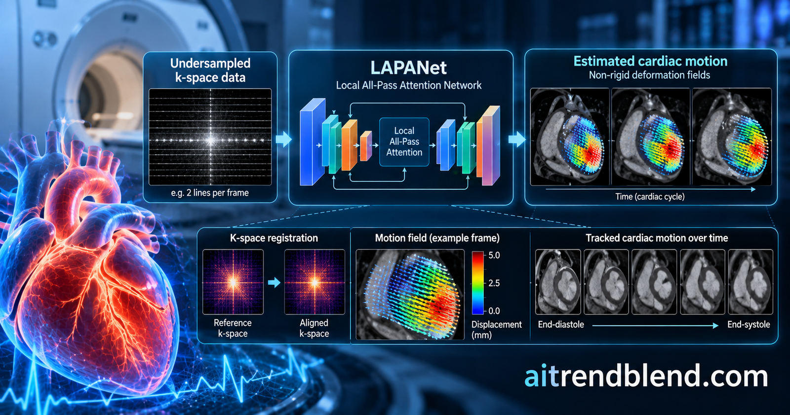
Think of a patient lying in a cardiac MRI scanner with an irregular heartbeat. The standard cine protocol asks for repeated breath holds and stitches the picture together from many beats, so an irregular rhythm smears the very thing the cardiologist wants to see. A faster, real time scan would show each beat as it happens. It would also be so heavily undersampled that every frame arrives full of streaks, and the streaks make it hard to work out how the heart wall is actually moving.
A group at the University of Tübingen, led by Aya Ghoul and Thomas Küstner with Kerstin Hammernik and Daniel Rueckert from Munich, went after that problem from an unusual side. Their network never reconstructs an image at all. It reads the raw frequency data directly and outputs a motion field. The open access paper in Medical Image Analysis calls it LAPANet. This article explains how it works, what the evidence supports, and where the paper’s own caveats begin.
Key points
- LAPANet estimates non rigid cardiac motion straight from accelerated multi coil k space. It needs no intermediate reconstruction, no prior scan and no ground truth motion fields.
- It was trained on cine MRI from 134 people and tested on 25 held out subjects. Motion was recovered from as few as 2 lines per frame on a Cartesian trajectory (acceleration 78, 4.24 ms per frame) and 3 spokes per frame on a radial one (acceleration 104, 4.99 ms).
- Up to acceleration 78 the mean target registration error stayed at or below 2.8 mm for initial misalignments of up to 7.2 mm. Image based competitors degraded as acceleration rose, and Elastix failed to converge at high accelerations.
- Inference takes about 30 ms per frame pair and 7.78 GB of GPU memory. The earlier k space method LAPNet needs about 2 minutes and more than 300 GB for the same task.
- Undersampling was simulated from fully sampled scans, the data are 2D from one scanner, and there is no independent motion reference such as tagging. The authors present it as a method under validation and not as a clinical tool.
Medical disclaimer. This article explains a published research paper. It is not medical advice, diagnosis or treatment, and the method described here is a research technique, not an approved clinical product. Any question about your heart or an MRI result belongs with a qualified cardiologist or radiologist.
Why moving organs are hard to scan
MRI is slow because it does not take a picture the way a camera does. It measures the image one line of frequency data at a time, filling a space that physicists call k space, and only then turns that space into an image with a Fourier transform. Every line costs time. The heart moves all the time, so the scan has to either freeze the motion with tricks, such as triggering, breath holds and navigators, or average over it.
The paper opens with a sobering figure. Nearly 20 percent of clinical MRI exams involve repeated sequences because of motion degraded images, at an annual cost the authors put at about 115,000 dollars per scanner, citing work from 2015. Patient movement contributes ghosting, blurring and ringing, and the usual fixes depend on external sensors or on the patient being able to cooperate. Irregular rhythms and patients who cannot hold their breath are the hardest cases, and they are also the ones who most need a good scan.
The alternative is to scan so fast that the heart barely moves within a frame. That means acquiring only a sliver of k space per frame, a setting called high undersampling. The price is aliasing. The missing lines do not simply make the picture blurry, they fold ghost copies of the anatomy on top of itself. An estimate of motion needs to match points between a moving frame and a fixed one, and ghosts corrupt exactly the structures those matches depend on.
Here is where it gets interesting. The usual workflow reconstructs first and registers second. The registration step then inherits every reconstruction artifact. The authors ask a blunt question. If undersampling damages the image so badly, why go through the image at all?
The idea that motion is a phase shift
The physics behind the answer is old and elegant. Shift an image by a few pixels and its Fourier transform does not change in magnitude. It only picks up a phase that grows linearly with frequency. So a translation in image space is a multiplication by a complex exponential in k space.
The second expression is called an all pass filter, because it changes the phase of every frequency and leaves the magnitude alone. Real cardiac motion is not one global translation, of course. The Local All Pass idea, developed by Gilliam, Küstner and Blu in 2016, treats the image as a patchwork. Inside a small window the motion is approximately a translation, which means approximately a phase shift, and the full non rigid motion is assembled from many overlapping local estimates.
That is a clean and interpretable link between deformation and spectrum. It has a cost, and the paper spells it out. The deformation must be assembled from windowed pieces, so results depend on window choice, and accuracy falls when undersampling leaves only a few samples inside each window. A deep learning version of the idea, LAPNet from 2021, learned the estimation from patches but still relied on hand built tapering windows, supervised training with synthetic motion fields and a heavy compute bill.
LAPANet drops the patches. The authors observe that even under severe undersampling, global frequency patterns and the different phase signature of every receiver coil survive. So instead of cutting k space into local windows by hand, the network looks at the whole thing and learns its own multi scale decomposition. Spatially varying motion is then encoded implicitly in the hierarchy of learned features.
The phase shift picture explains why the approach is plausible, and the network is what makes it practical. The physics says motion lives in the phase of k space. The learning part replaces hand tuned windows with attention over the whole spectrum.
Inside the network
The model works on four resolution levels. Its input is a pair of k spaces, a fixed frame and a moving frame, each resolved by coil. The authors compress the receiver array to 16 virtual coils with a singular value decomposition, crop to 160 by 160, and stack the real and imaginary parts of both frames into one real valued image with many channels. An inverse zero frequency shift then moves the low frequencies from the center to the corners, a trick the paper says helps local features and speeds convergence.
Three building blocks carry the design.
Global Residual Blocks look at the full stacked k space at each level. Inside, a self attention step built from depthwise convolutions preserves spatial context without positional encoding and attends across channels, where coil weighting and fixed versus moving information are stored. An attention weighted squeeze and excitation step then recalibrates channels. The output is a learned, data driven replacement for the phase modulated tapering windows of earlier work, at coarser scales for the deeper levels.
Encoder and decoder blocks combine those global features with convolutional features. Each holds a Channel Integration Module and a Dilated Fusion Module. The first reweights channels with attention, the second runs parallel dilated convolutions with dilations of 1, 2 and 4 to grow the receptive field cheaply. Dilation matters here because a single frequency sample touches every pixel of the image, so local kernels see little of the structure by themselves.
Motion Attention Modules sit at the end of each decoder level. They refine the current flow estimate by combining it with the previous coarser estimate and then weighting each of the two flow channels with its own learned attention map. The network emits four flow fields, from coarse to fine. Only the finest is used at inference. The others serve as deep supervision, meaning they get their own loss terms during training. A separate head predicts one global translation from the bottleneck, which gives the encoder an early signal about bulk motion.
The model has 17.2 million trainable parameters. For comparison, training took about 120 hours, roughly 2 hours per epoch for 60 epochs, on two NVIDIA V100 graphics cards, using AdamW with a learning rate of 0.0001, weight decay of 0.001, a batch size of 32 and cosine annealing. Hyperparameters were chosen by random search on the validation subjects.
Learning without a motion answer key
No dataset of true cardiac deformation exists, so the authors train without one. The idea is to let the fully sampled images act as the answer. During training each subject contributes a fully sampled pair, and the network only ever sees accelerated versions of it. The fully sampled k spaces are turned into coil combined images with the adjoint of the MRI encoding operator, which models coil sensitivities and the Fourier transform.
The main loss then asks whether warping the moving image with the predicted motion reproduces the fixed image, with a bounding box around the ventricles so the heart drives the loss and not the quiet background. This is the classic photometric loss of unsupervised registration.
A second loss is new. The k space magnitude consistency term compares the magnitudes of the fixed k space and the k space of the warped moving image. Magnitude is unaffected by the phase of a translation, so this term gives the network global structural guidance without asking it to match complex valued data exactly. The authors contrast it with the data consistency terms used in reconstruction, which enforce identity in complex k space.
A smoothness term keeps the field locally coherent, using the L1 norm of its spatial gradients. A translation loss trains the global translation head to align the two frames by a single shift.
The weights are 0.5 for the translation term, 0.05 for magnitude consistency and 0.01 for smoothness, all chosen by random search on the validation set. Everything is differentiable through the warp and the Fourier operators, so one optimizer trains the whole system end to end.
Stop for a moment on what that training scheme requires. The loss is computed against fully sampled data, and the authors say this is deliberate, to give the network high quality targets. At test time the network sees only accelerated k space. So the method does not need fully sampled data when it is used, yet it does need them when it is trained. The paper lists this as a limitation, and for cine MRI it is a mild one, because a conventional protocol with modest acceleration can supply the full data. It would be a harder problem for sequences where full coverage is physically impossible.
“the training objective requires access to fully sampled data, which are often not available in clinical routine acquisitions”Ghoul and colleagues, Medical Image Analysis, 2027
The data and the acceleration settings
The dataset was acquired in house at Tübingen on a 1.5 tesla Siemens MAGNETOM Aera. It contains multi slice short axis 2D cine scans, recorded with a balanced steady state free precession sequence during 15 second breath holds. Table 1 condenses the cohort and the protocol.
| Item | Detail |
|---|---|
| Participants | 134 in total, 96 patients with suspected cardiovascular disease (age 45 ± 17 years, 24 female) and 38 healthy subjects (age 32 ± 6 years, 14 female) |
| Split by subject | Training 97 (25 healthy, 72 patients), validation 12 (4 healthy, 8 patients), test 25 (9 healthy, 16 patients) |
| Sequence | 2D bSSFP cine, short axis, TE 1.06 ms, TR 2.12 ms, flip angle 52 degrees, 15 second breath holds |
| Resolution | 1.9 by 1.9 mm in plane, 8 mm slices, matrix 176 by 132 to 192 by 180, 25 cardiac phases, temporal resolution 22 to 48 ms |
| Image pairs | 647,500 for training and 171,875 for testing, all fixed and moving frame pairs across the cardiac cycle |
| Reference masks | Left and right ventricles segmented with Segment software and then corrected manually |
| Undersampling | Retrospective. Cartesian masks follow VISTA, radial masks use golden angle sampling |
Table 1. Dataset and protocol, condensed from Section 2.3 of the paper. The age entries are mean and standard deviation.
The word retrospective matters. The accelerated frames were not acquired at high speed. They were created afterwards by discarding lines or spokes from fully sampled data. An acceleration factor R is the number of lines in the fully sampled grid divided by the number kept, so 156 lines reduced to 2 gives R of 78 and 310 radial spokes reduced to 3 gives about R of 104. During training, accelerations ranged from fully sampled up to the highest tested values, 78 for Cartesian and 104 for radial. One model was trained for each sampling trajectory and handles every acceleration rate, which means the acceleration does not have to be known or chosen in advance.
What happens at two lines per frame
The comparison set is broad. The authors evaluate against conventional registration methods (Elastix, SyN, LDDMM and the original LAP) and two trained image based networks, VoxelMorph and GMA RAFT, the latter from the same group’s 2024 work. The earlier k space network LAPNet gets a separate qualitative comparison. Image based methods get the best treatment the paper knows how to give them, a single model per trajectory trained across accelerations, with hyperparameters tuned by random search on the same validation subjects.
Two downstream tasks measure success. The first is image alignment, the normalized root mean square error between the fully sampled fixed frame and the fully sampled moving frame warped with the motion that was estimated from accelerated data. The second is anatomy, registering the ventricular masks between end systole and end diastole, the two phases with the largest deformation, and scoring Dice overlap and Hausdorff distance on the blood pool of the right ventricle and the cavity and myocardium of the left.
A detail worth pausing on. Motion is always estimated from accelerated k space, but the metrics are computed on fully sampled images and masks. So the score reflects motion quality, not image quality, and it is not contaminated by the artifacts that hurt the image based competitors. That is the right design. It also means the test mixes a simulated acceleration with a clean evaluation target.
| Setting | Lines or spokes per frame | Acceleration R | What the paper reports for LAPANet |
|---|---|---|---|
| Cartesian VISTA | 156 down to 2 | 1 up to 78 | Mean target registration error at or below 2.8 mm (1.5 pixels) for initial misalignments up to 7.2 mm. HDD p = 0.801 and DSC p = 0.962 across accelerations |
| Radial golden angle | 310 down to 3 | 1 up to 104 | Mean HDD at or below 3.3 mm (1.7 pixels), mean DSC 0.81. HDD p = 0.353 and DSC p = 0.996 across accelerations |
Table 2. Headline accuracy across acceleration factors on the 25 test subjects, from Sections 3.1 and 4 of the paper. The p values come from one way ANOVA testing whether the metric changes with acceleration.
Read the pattern across accelerations. LAPANet held its scores essentially flat from fully sampled data up to acceleration 78 in Cartesian sampling and up to 104 in radial sampling. GMA RAFT did well when the data were fully sampled, then started to deteriorate beyond acceleration 31.2. VoxelMorph trailed from the start, and Elastix could not produce estimates at all for the highest accelerations, because it failed to converge. The image based methods failed in the way the authors predicted. Their error grew as aliasing artifacts got worse, and the difference from LAPANet was statistically significant for the competitors at the highest accelerations.
The paper adds qualitative figures for a patient with suspected right ventricular cardiomyopathy and for a healthy subject. LAPANet concentrates motion on the heart against a still background, while GMA RAFT and VoxelMorph produce diffuse flow as streaks take over. SyN and LDDMM produce spatially dispersed fields that follow the undersampling artifacts. Those pictures are persuasive, and they are also the kind of evidence a reader should weigh lightly next to numbers.
A caution about those p values
The ANOVA results need careful reading. LAPANet shows no significant change in HDD or DSC across accelerations, and the authors read that as stability. Two points temper it. A test that finds no significant difference is not proof of equivalence, especially when the metric is itself coarse. And the test set contains 171,875 image pairs from only 25 subjects. Pairs from the same person are strongly correlated, so the effective sample size is much closer to 25 than to 171,875. The paper says it computed the mean and standard deviation on all test image pairs, and it does not describe any adjustment for clustering within subjects. That is our observation and not a statement from the authors, yet it bears on how firmly to read the significance stars in the boxplots.
The consistent trend across metrics, trajectories and baselines is the strongest evidence here, stronger than any single p value. Every image based method lost ground as acceleration rose and LAPANet did not. A reader should trust the direction of that gap more than the exact significance levels.
Speed, memory and the real time claim
Efficiency is the second headline. LAPANet estimates the motion for one pair of frames in about 30 ms on a GPU using 7.78 GB of memory. The image based GMA RAFT needs about 70 ms and 2.12 GB, and VoxelMorph needs 1.44 GB. The big contrast is with LAPNet, the earlier k space method with a similar number of parameters. The hard coded tapering operations over small windows and strides send its inference to roughly 2 minutes and more than 300 GB of GPU memory for one bidirectional cine registration.
| Method | Inference per frame pair | GPU memory | Input domain |
|---|---|---|---|
| LAPANet | about 30 ms | 7.78 GB | K space |
| GMA RAFT | about 70 ms | 2.12 GB | Image |
| VoxelMorph | not stated in the main text | 1.44 GB | Image |
| LAPNet | about 2 minutes | more than 300 GB | K space |
Table 3. Computational cost, from Section 3.2 of the paper. Full tables of training time, FLOPs and parameters are in the supplementary material.
The authors summarize the LAPNet comparison as a 4,000 times speedup, a 600 times reduction in operations and a 40 times reduction in memory. They also report that LAPANet scales linearly with spatial size, that memory grows sub linearly with coil count, and that removing the Channel Integration, Motion Attention or Dilated Fusion modules would save less than 5 percent of peak memory. Those are design claims about the architecture. The numbers behind them sit in a supplementary table.
Now the subtle part. The abstract speaks of estimation at sub 5 ms temporal resolution, and the paper calls inference times suitable for online deployment. Both statements are true, yet they describe different clocks. The 4.24 ms at acceleration 78 is how long one frame takes to acquire, two lines at a repetition time of 2.12 ms each. The 30 ms is how long the network needs to process a frame pair. By our arithmetic, which is ours and not the paper’s, the network would fall behind an acquisition that delivers a new frame every 4 to 5 ms by a factor of about six or seven, unless the estimation is run on a subset of frame pairs, batched, or spread across several devices. Real time use is plausible, and this paper does not demonstrate a live pipeline.
Which parts of the design really matter
Ablation studies are where a paper shows it understands its own model. The authors removed each major block in turn, changed the loss and varied the input, using radial sampling at fully sampled data and accelerations of 31.2, 78 and 104.
- Architecture. Removing the Global Residual Block, the Dilated Fusion Module, the Channel Integration Module or the Motion Attention Module each degraded results across metrics and accelerations.
- Losses. Dropping the k space magnitude consistency term or the global translation loss hurt, and so did computing the loss on coil combined data in place of coil resolved data. In a simulation with Elastix derived reference motion, the magnitude term improved endpoint error and angular error, with a modest effect on fully sampled data and a larger effect at higher acceleration.
- Explicit tapering. Adding the old phase modulated tapering in front of the Global Residual Blocks did not help at low and medium acceleration, and hurt at high acceleration. At acceleration 78 the proposed design scored a normalized error of 0.08 ± 0.02 and a Hausdorff distance of 2.62 ± 0.54 mm against 0.09 ± 0.03 and 2.96 ± 0.79 mm with tapering. At acceleration 104 the pairs were 0.08 ± 0.02 with 2.6 ± 0.51 mm against 0.09 ± 0.03 with 2.88 ± 0.77 mm.
- Coils. Sixteen coil resolved data beat more compressed versions and showed no significant difference from 24 coils at high acceleration, so sensitivity diversity matters more than channel count.
- Input domain. The identical architecture fed with images instead of k space failed to learn reliable motion, even on fully sampled data, producing incoherent fields with non physical spikes.
That last result is the most striking and deserves a moment. The authors explain it this way. In the image domain the network must implicitly invert the variable, nonlinear artifacts of undersampling before it can register anything, which confounds inference. In k space, motion shows up as phase modulation that stays consistent whatever the sampling pattern. It is an appealing argument. It is also one result from one architecture, evaluated qualitatively on a patient with suspected myocarditis in the supplement, and it sits oddly next to the fact that strong image based registration networks work well on fully sampled images. Our own toy experiment in the code section, which is tiny and should not be over read, did not reproduce the gap.
“the network must implicitly invert the variable, nonlinear artifacts of undersampling, to perform an image registration”Ghoul and colleagues, Medical Image Analysis, 2027, on why image inputs struggle
What the network pays attention to
The interpretability analysis uses integrated gradients, which trace each output back to the input samples that influenced it. The attribution maps concentrate on the center of k space, the low frequencies, and show negative attribution in the periphery, in both Cartesian and radial sampling and at every acceleration. Average line profiles and noise power spectra tell the same story. As acceleration rises, high frequencies count for less and low frequencies dominate, which the authors describe as the network acting like a low pass filter that suppresses high frequency noise.
This is useful beyond curiosity. The center of k space carries the coarse shape and most of the signal energy, and the finding suggests how a sampling pattern could be designed around motion estimation, spending a limited budget on the frequencies the network actually uses. The authors note this as a route to adaptive sampling. It remains a hypothesis here, because no such pattern was tested.
The clinical translation gap
What would it take to move this from a research result to something a cardiac MRI service could use? The paper is upfront that it has not gotten there, and the gaps are worth listing in plain terms.
First, the accelerated data are simulated. A real accelerated acquisition has its own contrast behavior, eddy current effects and noise, and the retrospective approach sidesteps all of them. Second, the evaluation anchors on ventricle masks between end systole and end diastole. That is a reasonable proxy for gross motion and it says little about regional strain, torsion or the fine detail of wall motion. The authors plan to benchmark against independent references such as tagging and DENSE, and they have not yet done it.
Third, everything is two dimensional. The paper states that cardiac dynamics are three dimensional, with shear, torsion and through plane displacement, and that through plane motion, especially near the apex and base, creates errors the 2D data cannot observe. Its own conclusion is that the estimated fields should be read as projections of the true motion.
“The estimated motion fields should thus be interpreted as 2D projections of the underlying 3D cardiac motion.”Ghoul and colleagues, Medical Image Analysis, 2027
Fourth, the method estimates motion frame by frame. It ignores smoothness between frames, which can cost temporal consistency in dynamic sequences. The authors point to recurrent networks, bidirectional flow learning, groupwise objectives and spatio temporal regularization as fixes.
Regulatory and safety notes
The paper does not discuss regulation, so this paragraph is our own reading. Software that estimates motion for diagnosis or to guide an intervention would very likely be treated as a medical device in most jurisdictions, with evidence requirements well beyond retrospective cine data from one scanner. The authors mention applications such as MR guided catheterization and radiotherapy, where a motion estimate could steer a tool or a beam. That is exactly where an undetected error in an out of distribution patient would matter most, and it is why a prospective study with an independent reference comes before any such use. Until then, the outputs are research quantities, and any clinical conclusion about a heart should come from a clinician reading the standard images.
Where the idea could travel
The obvious neighbor is motion corrected reconstruction. A fast motion estimate gives a reconstruction algorithm the deformation it needs to combine many undersampled frames into one sharp image. On this site, our piece on cardiac MRI reconstruction with KGMgT covers the reconstruction side of the story, and our look at guided reconstruction of brain and knee MRI shows the same pressure to do more with fewer samples. LAPANet works the other way around. It skips the image and asks whether the motion was ever recoverable without one.
If you want the image domain view of the same clinical question, our article on CardioMorphNet and Bayesian cardiac motion estimation tracks 3D heart motion from reconstructed images with shape guidance. Reading the two together makes the trade clear. The image route uses anatomical shape priors that only exist once you have a picture. The k space route gives up the picture in exchange for robustness when the picture is poor.
Downstream tasks benefit from motion too. Ventricular function measures rest on contours and volumes, and our analysis of why heart masks do not improve ejection fraction prediction shows how sensitive those measures are to small tracing errors. Cine segmentation in congenital disease appears in our article on segmenting single ventricle hearts from cine MRI. The same physics first thinking shows up in our piece on quantitative T1 and T2 maps from routine brain MRI, where a forward model of the scanner supplies the supervision. More studies of this kind sit in our Medical AI section.
Limitations, sample size and bias
The authors write a candid limitations discussion, and this section builds on it, adding points the numbers suggest.
- Small, single center cohort. The 134 participants come from one hospital and one 1.5 tesla scanner. The test set has 25 subjects, 9 healthy and 16 patients, and the main text gives no breakdown by disease. Performance on other vendors, field strengths, sequences and patient populations is unknown, and the authors list larger prospective cohorts as future work.
- Healthy and younger controls. The healthy group averages 32 years against 45 for the patients, so disease and age are partly confounded, and the main text reports no results by group.
- Simulated acceleration. All accelerated data are retrospectively undersampled from fully sampled cine. Real time acquisitions and free breathing data were not tested.
- No independent motion reference. Accuracy is judged through image similarity and ventricle mask overlap. There is no comparison with tagging or DENSE, so regional strain accuracy is untested.
- Two dimensional motion only. Through plane motion is unobservable and appears as residual error.
- Fully sampled data needed for training. The loss uses fully sampled k space. Sequences where full coverage is impossible would need a different training scheme, which the authors propose to study.
- Frame by frame estimation. There is no temporal consistency constraint across a cine series.
- Latency versus frame rate. About 30 ms per frame pair exceeds the 4 to 5 ms acquisition time per frame at the highest accelerations.
- Data access. The paper states that data will be made available on request, so independent replication on the same cohort is not open. The code is public on GitHub.
- Disclosures. The authors declare no known competing financial interests, and the work was supported by the German Research Foundation under the Excellence Strategy.
A PyTorch reconstruction of LAPANet
The authors released their own implementation in a public GitHub repository, and anyone doing real work should start there. What follows is our independent reconstruction from the paper’s text, figures and equations, written so every moving part sits in one readable file. It has never touched patient data.
The file holds the centered Fourier helpers and the multi coil encoding operator with its adjoint, the Global Residual Block with its channel self attention and attention weighted squeeze and excitation, the Channel Integration and Dilated Fusion modules, encoder and decoder blocks, the Motion Attention Module, the full four level network with its global translation head, the warp, the complete loss of Equations 4 to 8, a synthetic contracting heart phantom with known motion, Cartesian undersampling, and a smoke test. Every place where the paper leaves a detail open is marked DESIGN CHOICE. It needs Python 3 and PyTorch 2, and it runs on a CPU.
"""
lapanet_reference.py
Educational reconstruction of LAPANet, the Local All Pass Attention Network for
non rigid registration directly in k space, from
"Learning efficient non rigid registration in k space for accelerated Magnetic Resonance Imaging"
(Ghoul et al., Medical Image Analysis 115, 2027, 104296). Paper DOI 10.1016/j.media.2026.104296.
The authors' own code is at https://github.com/lab-midas/LAPANet and is the place to start for real work.

This file is an independent, unvalidated reconstruction from the paper's text, figures and equations.
Everything the paper leaves open is marked DESIGN CHOICE. It was never run on patient data.

Contents
  1. Centered FFT helpers, the multi coil forward operator A and its adjoint A^H.
  2. The network. Global Residual Blocks (GRB) with a channel self attention and an
     attention weighted squeeze and excitation, encoder and decoder blocks built from a
     Channel Integration Module (CIM) and a Dilated Fusion Module (DFM), and Motion
     Attention Modules (MAM) that emit four multi scale flow fields plus a global translation.
  3. The training loss (Eqs 4 to 8), a bilinear warp, and helpers.
  4. A synthetic beating heart phantom with known motion, Cartesian undersampling, and a smoke test
     that trains a small model and compares k space input with image input.
Requires Python 3 and PyTorch 2. Runs on CPU.
"""
import math
from typing import List, Sequence, Tuple

import torch
import torch.nn as nn
import torch.nn.functional as F

# ----------------------------------------------------------------------------
# 1. FFT helpers and the multi coil encoding operator
# ----------------------------------------------------------------------------
def fft2c(x: torch.Tensor) -> torch.Tensor:
    """Centered orthonormal 2D FFT over the last two dims."""
    return torch.fft.fftshift(torch.fft.fft2(torch.fft.ifftshift(x, dim=(-2, -1)), norm="ortho"), dim=(-2, -1))


def ifft2c(k: torch.Tensor) -> torch.Tensor:
    return torch.fft.fftshift(torch.fft.ifft2(torch.fft.ifftshift(k, dim=(-2, -1)), norm="ortho"), dim=(-2, -1))


def forward_op(img: torch.Tensor, smaps: torch.Tensor) -> torch.Tensor:
    """A. Image (B,H,W) complex and sensitivities (B,C,H,W) to coil k space (B,C,H,W)."""
    return fft2c(img[:, None] * smaps)


def adjoint_op(k: torch.Tensor, smaps: torch.Tensor) -> torch.Tensor:
    """A^H. Coil k space to a coil combined complex image (B,H,W), Eq 3."""
    return (ifft2c(k) * smaps.conj()).sum(dim=1)


# ----------------------------------------------------------------------------
# 2. Network
# ----------------------------------------------------------------------------
def conv(cin, cout, k=3, d=1):
    return nn.Conv2d(cin, cout, k, padding=d * (k // 2), dilation=d)


class ChannelSelfAttention(nn.Module):
    """Self attention across the channel dimension. Queries, keys and values come from depthwise
    convolutions, which keeps spatial context without positional encoding, and the attention map is
    C by C, so cost grows linearly with the number of pixels. DESIGN CHOICE: the paper describes
    depthwise Q, K, V and linear time attention but not the exact form, so this follows the
    transposed attention pattern."""

    def __init__(self, c: int):
        super().__init__()
        self.q = nn.Conv2d(c, c, 3, padding=1, groups=c)
        self.k = nn.Conv2d(c, c, 3, padding=1, groups=c)
        self.v = nn.Conv2d(c, c, 3, padding=1, groups=c)
        self.temp = nn.Parameter(torch.ones(1))

    def forward(self, x):
        b, c, h, w = x.shape
        q = F.normalize(self.q(x).flatten(2), dim=-1)
        k = F.normalize(self.k(x).flatten(2), dim=-1)
        v = self.v(x).flatten(2)
        attn = torch.softmax(q @ k.transpose(1, 2) * self.temp, dim=-1)      # (B, C, C)
        return (attn @ v).view(b, c, h, w) + x


class AttnSqueezeExcite(nn.Module):
    """Attention weighted Squeeze and Excitation. A softmax over space pools each channel into one
    descriptor, then a small bottleneck produces sigmoid channel weights (Fig 2)."""

    def __init__(self, c: int):
        super().__init__()
        self.score = nn.Conv2d(c, 1, 1)
        hidden = max(3, c // 2)
        self.fc = nn.Sequential(nn.Conv2d(c, hidden, 1), nn.SiLU(), nn.Conv2d(hidden, c, 1), nn.Sigmoid())

    def forward(self, x):
        w = torch.softmax(self.score(x).flatten(2), dim=-1)                  # (B, 1, HW)
        desc = (x.flatten(2) * w).sum(-1)[..., None, None]                   # (B, C, 1, 1)
        return x * self.fc(desc)


class GlobalResidualBlock(nn.Module):
    """GRB. Learns a multi resolution representation of the full stacked k space. It replaces the
    hand built phase modulated tapering windows of earlier k space methods. Work is done at full
    resolution and then max pooled by the level's factor."""

    def __init__(self, cin: int, cout: int, pool: int):
        super().__init__()
        self.cross = conv(cin, cout)
        self.main = nn.Sequential(nn.GroupNorm(1, cin), nn.SiLU(), conv(cin, cout), ChannelSelfAttention(cout),
                                  nn.SiLU(), conv(cout, cout, d=2), AttnSqueezeExcite(cout))
        self.pool = nn.MaxPool2d(pool) if pool > 1 else nn.Identity()

    def forward(self, x):
        return self.pool(self.cross(x) + self.main(x))


class CIM(nn.Module):
    """Channel Integration Module. Conv and SiLU stacks with one dilated conv, then an attention
    residual unit. DESIGN CHOICE: exact layer order follows Fig 3 loosely."""

    def __init__(self, c: int):
        super().__init__()
        self.stack = nn.Sequential(conv(c, c), nn.SiLU(), conv(c, c), nn.SiLU(), conv(c, c, d=2), nn.SiLU())
        self.attn = ChannelSelfAttention(c)
        self.res = nn.Sequential(conv(c, c), nn.SiLU())

    def forward(self, x):
        y = self.stack(x)
        return y + self.res(self.attn(y))


class DFM(nn.Module):
    """Dilated Fusion Module. Parallel 3 by 3 convolutions with dilations 1, 2 and 4 widen the
    receptive field, then a fusion conv and a residual connection with group normalization."""

    def __init__(self, c: int):
        super().__init__()
        self.branches = nn.ModuleList([nn.Sequential(conv(c, c, d=d), nn.BatchNorm2d(c), nn.SiLU()) for d in (1, 2, 4)])
        self.fuse = nn.Sequential(conv(3 * c, c), nn.BatchNorm2d(c), nn.SiLU())
        self.norm = nn.GroupNorm(1, c)

    def forward(self, x):
        y = self.fuse(torch.cat([b(x) for b in self.branches], dim=1))
        return self.norm(x + y)


class EncoderBlock(nn.Module):
    def __init__(self, cin: int, cgrb: int, cout: int):
        super().__init__()
        self.proj = nn.Sequential(nn.GroupNorm(1, cin + cgrb), conv(cin + cgrb, cout), nn.SiLU())
        self.cim, self.dfm = CIM(cout), DFM(cout)

    def forward(self, x, grb):
        return self.dfm(self.cim(self.proj(torch.cat([x, grb], dim=1))))


class DecoderBlock(nn.Module):
    def __init__(self, cin: int, cskip: int, cout: int):
        super().__init__()
        self.proj = nn.Sequential(conv(cin + cskip, cout), nn.SiLU())
        self.cim, self.dfm = CIM(cout), DFM(cout)

    def forward(self, x, skip):
        x = F.interpolate(x, scale_factor=2, mode="nearest")
        return self.dfm(self.cim(self.proj(torch.cat([x, skip], dim=1))))


class MotionAttentionModule(nn.Module):
    """MAM. Turns decoder features into a 2 channel flow estimate, adds the upsampled estimate of the
    previous level, and weights each flow channel with its own learned [0, 1] attention map.
    DESIGN CHOICE: the paper upsamples inside the MAM, here the decoder block already upsamples, so the
    MAM keeps the decoder's resolution. Flow is expressed in full resolution pixels at every level."""

    def __init__(self, c: int):
        super().__init__()
        self.est = nn.Sequential(conv(c, c), nn.SiLU(), conv(c, c), nn.SiLU(), conv(c, 2))
        self.mask = nn.ModuleList([nn.Sequential(conv(2, 8), nn.SiLU(), conv(8, 1), nn.Sigmoid()) for _ in range(2)])

    def forward(self, feat, prev=None):
        u = self.est(feat)
        if prev is not None:
            u = u + F.interpolate(prev, size=u.shape[-2:], mode="bilinear", align_corners=False)
        return torch.cat([u[:, i:i + 1] * self.mask[i](u) for i in range(2)], dim=1)


class LAPANet(nn.Module):
    """Four level U shaped network. Input is the stacked real and imaginary parts of the coil resolved
    fixed and moving k spaces, shape (B, 4 * n_coils, H, W), with H and W divisible by 16.
    Returns four flow fields from coarse to fine and a global translation."""

    def __init__(self, n_coils: int = 16, widths=(16, 32, 64, 192), bottleneck=384, grb_widths=(4, 16, 32, 128)):
        super().__init__()
        cin = 4 * n_coils
        self.grbs = nn.ModuleList([GlobalResidualBlock(cin, g, 2 ** i) for i, g in enumerate(grb_widths)])
        self.enc = nn.ModuleList()
        prev = cin
        for i, (w, g) in enumerate(zip(widths, grb_widths)):
            self.enc.append(EncoderBlock(prev, g, w)); prev = w
        self.bott = nn.Sequential(conv(widths[-1], bottleneck), nn.SiLU(), CIM(bottleneck))
        self.dec = nn.ModuleList()
        dprev = bottleneck
        for w, skip in zip(reversed(widths), reversed(widths)):
            self.dec.append(DecoderBlock(dprev, skip, w)); dprev = w
        self.mams = nn.ModuleList([MotionAttentionModule(w) for w in reversed(widths)])
        self.trans = nn.Conv2d(bottleneck, 2, 1)   # global translation u_t from the bottleneck

    def forward(self, x):
        skips, h = [], x
        for i in range(4):
            h = self.enc[i](h, self.grbs[i](x))
            skips.append(h)
            h = F.max_pool2d(h, 2)
        b = self.bott(h)
        # DESIGN CHOICE: the paper max pools the bottleneck over 5 by 5 at its 160 by 160 input,
        # an adaptive max pool gives the same global 1 by 1 result at any input size.
        u_t = F.adaptive_max_pool2d(self.trans(b), 1)[..., 0, 0]       # (B, 2)
        flows, prev, d = [], None, b
        for i in range(4):
            d = self.dec[i](d, skips[3 - i])
            prev = self.mams[i](d, prev)
            flows.append(prev)
        return flows, u_t


# ----------------------------------------------------------------------------
# 3. Warping and the training loss (Eqs 4 to 8)
# ----------------------------------------------------------------------------
def warp(img: torch.Tensor, flow: torch.Tensor) -> torch.Tensor:
    """Bilinear backward warp, T(I_mov, u). img is (B,H,W) real or complex, flow is (B,2,H,W) in pixels
    with channel 0 along width and channel 1 along height."""
    if img.is_complex():
        return torch.complex(warp(img.real, flow), warp(img.imag, flow))
    b, h, w = img.shape
    ys, xs = torch.meshgrid(torch.arange(h, dtype=img.dtype), torch.arange(w, dtype=img.dtype), indexing="ij")
    gx = (xs[None] + flow[:, 0]) / (w - 1) * 2 - 1
    gy = (ys[None] + flow[:, 1]) / (h - 1) * 2 - 1
    return F.grid_sample(img[:, None], torch.stack([gx, gy], dim=-1), mode="bilinear",
                         padding_mode="border", align_corners=True)[:, 0]


def upsample_flow(u: torch.Tensor, size) -> torch.Tensor:
    """Bilinear upsampling to full resolution. Flow is already in full resolution pixels."""
    return F.interpolate(u, size=size, mode="bilinear", align_corners=False)


def grad_l1(u: torch.Tensor) -> torch.Tensor:
    """Eq 6. L1 norm of forward finite difference gradients. DESIGN CHOICE: the paper obtains the
    smoothness term from an anisotropic diffusion regularizer, a plain L1 gradient is used here."""
    return (u[..., 1:, :] - u[..., :-1, :]).abs().mean() + (u[..., :, 1:] - u[..., :, :-1]).abs().mean()


def lapanet_loss(flows, u_t, i_fix_fs, i_mov_fs, k_fix_fs, smaps, box, alpha=0.5, beta=0.05, gamma=0.01):
    """Total loss, Eq 8. i_fix_fs and i_mov_fs are the fully sampled coil combined complex images made with A^H,
    k_fix_fs is the fully sampled fixed k space, box is the heart bounding box mask (B,H,W).
    The translation loss (Eq 7) is added once and the photometric (Eq 4), k space magnitude consistency (Eq 5)
    and smoothness (Eq 6) terms are summed over the four resolution levels. Returns the total and its parts."""
    h, w = i_fix_fs.shape[-2:]
    mag_fix = i_fix_fs.abs()
    norm_k_fix = k_fix_fs.abs().pow(2).sum(1).sqrt()
    tr = u_t[:, :, None, None].expand(-1, -1, h, w)
    l_trans = (box * (mag_fix - warp(i_mov_fs.abs(), tr)).abs()).mean()                     # Eq 7
    l_photo = l_kmc = l_smooth = 0.0
    for u in flows:
        uf = upsample_flow(u, (h, w))
        warped = warp(i_mov_fs, uf)
        l_photo = l_photo + (box * (mag_fix - warped.abs()).abs()).mean()                  # Eq 4
        norm_k_w = forward_op(warped, smaps).abs().pow(2).sum(1).sqrt()
        l_kmc = l_kmc + (norm_k_fix - norm_k_w).abs().mean()                               # Eq 5
        l_smooth = l_smooth + grad_l1(u)                                                   # Eq 6
    total = alpha * l_trans + l_photo + beta * l_kmc + gamma * l_smooth
    parts = {"trans": l_trans, "photo": l_photo, "kmc": l_kmc, "smooth": l_smooth}
    return total, {k: float(v.detach()) for k, v in parts.items()}


def make_input(k_fix_us, k_mov_us, smaps, domain="kspace"):
    """Stack real and imaginary parts of the coil resolved fixed and moving inputs. The paper applies an
    inverse zero frequency shift so low frequencies sit at the corners (helps local features and
    convergence). domain='image' gives the zero filled image domain input used in the paper's ablation."""
    if domain == "image":
        k_fix_us, k_mov_us = ifft2c(k_fix_us) * smaps.conj(), ifft2c(k_mov_us) * smaps.conj()
    else:
        k_fix_us = torch.fft.ifftshift(k_fix_us, dim=(-2, -1)); k_mov_us = torch.fft.ifftshift(k_mov_us, dim=(-2, -1))
    return torch.cat([k_fix_us.real, k_fix_us.imag, k_mov_us.real, k_mov_us.imag], dim=1)


# ----------------------------------------------------------------------------
# 4. Synthetic beating heart phantom, undersampling, smoke test
# ----------------------------------------------------------------------------
def coil_maps(n_coils: int, size: int) -> torch.Tensor:
    """Smooth Gaussian sensitivity profiles around the field of view, normalized to unit sum of squares."""
    ys, xs = torch.meshgrid(torch.linspace(-1, 1, size), torch.linspace(-1, 1, size), indexing="ij")
    maps = []
    for c in range(n_coils):
        a = 2 * math.pi * c / n_coils
        cx, cy = 1.3 * math.cos(a), 1.3 * math.sin(a)
        mag = torch.exp(-((xs - cx) ** 2 + (ys - cy) ** 2) / 1.6)
        maps.append(torch.polar(mag, (xs * math.cos(a) + ys * math.sin(a)) * 0.8))
    m = torch.stack(maps)
    return m / m.abs().pow(2).sum(0, keepdim=True).sqrt().clamp_min(1e-6)


def phantom_pair(size: int, gen: torch.Generator):
    """Fixed and moving frames of a contracting ring (myocardium around a blood pool). The moving frame has all
    radii scaled by c, so the known flow from fixed to moving is (c - 1) times the offset from the centre,
    faded out away from the heart. Returns images, the true flow and a bounding box mask."""
    r = lambda lo, hi: float(lo + (hi - lo) * torch.rand(1, generator=gen))
    cx, cy = size / 2 + r(-4, 4), size / 2 + r(-4, 4)
    ri, ro, c = r(0.12, 0.17) * size, r(0.26, 0.31) * size, r(0.72, 0.9)
    ys, xs = torch.meshgrid(torch.arange(size, dtype=torch.float32), torch.arange(size, dtype=torch.float32), indexing="ij")
    dx, dy = xs - cx, ys - cy
    rho, theta = (dx ** 2 + dy ** 2).sqrt(), torch.atan2(dy, dx)

    def render(scale):
        ring = torch.sigmoid((rho - ri * scale) / 1.2) * torch.sigmoid((ro * scale - rho) / 1.2)
        blood = torch.sigmoid((ri * scale - rho) / 1.2)
        texture = 1 + 0.25 * torch.sin(3 * theta + 1.0) * torch.sigmoid((ro * scale - rho) / 1.2)
        return 0.9 * ring * texture + 0.45 * blood + 0.05

    fade = torch.sigmoid((1.5 * ro - rho) / 2.0)
    flow = torch.stack([(c - 1) * dx * fade, (c - 1) * dy * fade])
    box = (rho < ro * 1.4).float()
    return render(1.0), render(c), flow, box


def variable_density_mask(size: int, n_lines: int, gen: torch.Generator) -> torch.Tensor:
    """Cartesian mask keeping n_lines phase encode columns. The centre line is always kept and the others are drawn
    with a Gaussian preference for low frequencies. DESIGN CHOICE: a simple stand in for the VISTA design."""
    keep = {size // 2}
    p = torch.exp(-0.5 * ((torch.arange(size) - size // 2) / (size / 6)) ** 2); p[size // 2] = 0
    while len(keep) < n_lines:
        keep.add(int(torch.multinomial(p, 1, generator=gen)))
    m = torch.zeros(size, size); m[:, sorted(keep)] = 1
    return m


def make_batch(batch: int, size: int, n_coils: int, lines_choices: Sequence[int], gen: torch.Generator):
    maps = coil_maps(n_coils, size)[None].expand(batch, -1, -1, -1)
    fixs, movs, flows, boxes, kf_us, km_us, kf_fs = [], [], [], [], [], [], []
    for _ in range(batch):
        f, m, fl, bx = phantom_pair(size, gen)
        n = int(lines_choices[int(torch.randint(len(lines_choices), (1,), generator=gen))])
        mf, mm = variable_density_mask(size, n, gen), variable_density_mask(size, n, gen)
        kf = forward_op(f.to(torch.complex64)[None], maps[:1])[0]
        km = forward_op(m.to(torch.complex64)[None], maps[:1])[0]
        fixs.append(f); movs.append(m); flows.append(fl); boxes.append(bx)
        kf_us.append(kf * mf); km_us.append(km * mm); kf_fs.append(kf)
    st = lambda l: torch.stack(l)
    return dict(maps=maps, flow=st(flows), box=st(boxes), k_fix_us=st(kf_us), k_mov_us=st(km_us), k_fix_fs=st(kf_fs),
                i_fix_fs=adjoint_op(st(kf_fs), maps),
                i_mov_fs=adjoint_op(forward_op(st(movs).to(torch.complex64), maps), maps))


def endpoint_error(flow_pred: torch.Tensor, flow_true: torch.Tensor, box: torch.Tensor) -> float:
    """Mean endpoint error in pixels inside the heart box."""
    e = ((flow_pred - flow_true) ** 2).sum(1).sqrt()
    return float((e * box).sum() / box.sum())


def train(domain: str, steps: int = 120, size: int = 64, n_coils: int = 4, seed: int = 0, widths=(8, 16, 24, 32), bott=48):
    torch.manual_seed(seed)
    gen = torch.Generator().manual_seed(seed)
    net = LAPANet(n_coils, widths, bott, grb_widths=(4, 8, 12, 16))
    opt = torch.optim.AdamW(net.parameters(), lr=1e-3, weight_decay=1e-3)
    sched = torch.optim.lr_scheduler.CosineAnnealingLR(opt, steps)
    hist = []
    for s in range(steps):
        b = make_batch(6, size, n_coils, (size, 16, 8, 4, 2), gen)
        x = make_input(b["k_fix_us"], b["k_mov_us"], b["maps"], domain)
        flows, u_t = net(x)
        loss, parts = lapanet_loss(flows, u_t, b["i_fix_fs"], b["i_mov_fs"], b["k_fix_fs"], b["maps"], b["box"])
        opt.zero_grad(); loss.backward(); opt.step(); sched.step()
        hist.append(float(loss.detach()))
    return net, hist


@torch.no_grad()
def evaluate(net, domain: str, n_lines: int, size: int = 64, n_coils: int = 4, n_batches: int = 6, seed: int = 123):
    net.eval()
    gen = torch.Generator().manual_seed(seed)
    epes, base = [], []
    for _ in range(n_batches):
        b = make_batch(6, size, n_coils, (n_lines,), gen)
        flows, _ = net(make_input(b["k_fix_us"], b["k_mov_us"], b["maps"], domain))
        epes.append(endpoint_error(upsample_flow(flows[-1], (size, size)), b["flow"], b["box"]))
        base.append(endpoint_error(torch.zeros_like(b["flow"]), b["flow"], b["box"]))
    net.train()
    return sum(epes) / len(epes), sum(base) / len(base)


def smoke_test():
    torch.manual_seed(0)
    # 1. Shapes and parameter count at the paper's widths (16 coils, 160 by 160 input)
    big = LAPANet(n_coils=16)
    n_params = sum(p.numel() for p in big.parameters()) / 1e6
    flows, u_t = big(torch.randn(1, 64, 160, 160))
    assert [tuple(f.shape[-2:]) for f in flows] == [(20, 20), (40, 40), (80, 80), (160, 160)] and u_t.shape == (1, 2)
    print(f"paper width model, trainable parameters {n_params:.1f} million (paper reports 17.2 million)")
    # 2. Adjoint consistency, A^H A on a fully sampled image with unit sum of squares maps returns the image
    maps = coil_maps(4, 64)[None]
    img = torch.randn(1, 64, 64, dtype=torch.complex64)
    assert torch.allclose(adjoint_op(forward_op(img, maps), maps), img, atol=1e-4)
    # 3. Warping with the true flow should align the moving frame to the fixed one
    f, m, fl, bx = phantom_pair(64, torch.Generator().manual_seed(1))
    err_zero = float(((f - m).abs() * bx).mean())
    err_true = float(((f - warp(m[None], fl[None])[0]).abs() * bx).mean())
    assert err_true < 0.5 * err_zero
    print(f"phantom check  photometric error zero flow {err_zero:.3f}  true flow {err_true:.3f}")
    # 4. Train two small models, identical except for the input domain
    results = {}
    for domain in ("kspace", "image"):
        net, hist = train(domain)
        assert hist[-1] < hist[0]
        results[domain] = {n: evaluate(net, domain, n)[0] for n in (64, 8, 4, 2)}
        print(f"{domain:<7} loss {hist[0]:.3f} to {hist[-1]:.3f}   endpoint error in pixels at 64 / 8 / 4 / 2 lines  "
              + " / ".join(f"{results[domain][n]:.2f}" for n in (64, 8, 4, 2)))
    zero = evaluate(net, "image", 2)[1]
    print(f"zero flow baseline endpoint error {zero:.2f} pixels")
    print("smoke test passed")


if __name__ == "__main__":
    smoke_test()
The smoke test runs four checks and then a small experiment. It builds the network at the paper’s widths and confirms the four flow shapes, it checks that the adjoint operator recovers an image through unit sum of squares coil maps, it confirms that warping the phantom with its true flow cuts the photometric error, and it trains two small models that differ only in their input, one fed k space and one fed zero filled images, in the spirit of the paper’s input domain ablation.
Read these numbers as plumbing checks and nothing more. The full width model has 16.3 million parameters against the paper’s 17.2 million, close enough to suggest the layout is in the right neighborhood and far enough to confirm that some block details differ from the authors’. The toy trains for only 120 steps on 64 by 64 phantoms with 4 coils, and the motion is a single contraction, which is a far simpler problem than a beating human heart. Both models learn something, cutting the endpoint error from 2.78 pixels for a zero flow guess to about one pixel.
The interesting part is what did not happen. In this toy the image input model was slightly better than the k space model, and neither degraded visibly as the number of lines dropped from 64 to 2. That is the opposite of the paper’s headline contrast. It would be wrong to read it as a refutation. One seed, a few minutes of training and a motion model with essentially two free parameters cannot test a claim about real cardiac motion at 25 subjects scale. What it does show is that the paper’s finding is not trivially true of any network on any data, and that an honest replication needs real accelerated cine data and far longer training.
What this adds up to
The core achievement is a network that estimates non rigid cardiac motion directly from heavily undersampled multi coil k space, with no intermediate reconstruction, no prior scan and no ground truth motion fields. Trained on cine data from 134 people, it held its accuracy flat while image based baselines fell apart, down to 2 lines per frame in Cartesian sampling and 3 spokes in radial sampling. It did so in about 30 ms per frame pair and 7.78 GB of memory, against roughly 2 minutes and more than 300 GB for the earlier k space method.
The conceptual shift is to stop treating the image as the necessary intermediate. Medical imaging pipelines are built as sequences, acquire, reconstruct, analyze, and each stage inherits the flaws of the last. This paper asks which tasks can be done upstream of the picture, on the measurements themselves, and argues that motion is one of them because motion leaves a clean signature in phase. The paper’s ablation, where the same architecture on image inputs failed, is the boldest piece of evidence for that view.
The idea should travel to other fields that measure in a transform domain. Radar, ultrasound beamforming, computed tomography sinograms and spectroscopy all acquire signals whose physical structure survives undersampling better than their reconstructions do. The authors mention prostate, abdominal and musculoskeletal motion as natural next targets. What would carry over is a recipe, a physical model that says how the quantity of interest shows up in the raw data, plus an architecture with a global receptive field so every sample can talk to every other.
The remaining limitations are real, and the authors list most of them. The data come from one center, one scanner and 2D slices. The undersampling is simulated from fully sampled scans, training needs those fully sampled scans, no independent motion reference such as tagging or DENSE was used, and estimation runs frame by frame. The real time framing also deserves care, because 30 ms of inference per pair is slower than a frame that takes 4 to 5 ms to acquire. Neither is a flaw in the science. Each marks a step that still has to be taken before this leaves the lab.
The road ahead is laid out in the paper. The authors plan to learn directly from undersampled data, with multi mask consistency and proxy targets from pretrained reconstruction networks, to add temporal consistency through recurrent and bidirectional models, to extend to 3D volumes, and to benchmark against tagging and DENSE in larger prospective cohorts with different sequences and motion patterns. They also want to explore a foundation model for motion estimation. A fair next test for outsiders would be a real accelerated acquisition from a different scanner, on patients with irregular rhythms, because those are the cases the method is meant to serve.
A heartbeat has always been something MRI had to work around. This paper suggests it may also be something the raw data can report on directly, and it is honest enough to say how far that still is from a clinic.
Frequently asked questions
What does LAPANet do?
LAPANet is a deep learning framework from Ghoul and colleagues at the University of Tübingen that estimates non rigid motion between two cardiac MRI frames directly from accelerated multi coil k space. It produces a dense motion field without first reconstructing an image, and without needing a prior scan or ground truth motion fields.
Why estimate motion in k space instead of in images?
Heavy undersampling fills reconstructed images with aliasing artifacts that corrupt the structures image registration depends on. A translation in an image is a phase shift in k space, so motion leaves a signature that survives undersampling better than the picture does. In the paper, the same architecture fed with images failed to learn reliable motion, even on fully sampled data.
How was LAPANet trained without ground truth motion?
It is trained without any displacement labels. Fully sampled images and k spaces act as the target, and the loss combines a photometric term, a k space magnitude consistency term, a smoothness term and a global translation term over four resolution levels. Fully sampled data are needed for training but not when the trained model is used.
How accurate was it at high acceleration?
On 25 held out subjects, the mean target registration error stayed at or below 2.8 mm up to acceleration 78, which is 2 Cartesian lines per frame, for initial misalignments of up to 7.2 mm. With radial sampling up to acceleration 104, which is 3 spokes per frame, the mean Hausdorff distance stayed at or below 3.3 mm and the mean Dice score was 0.81. The undersampling was simulated from fully sampled scans.
Is it fast enough for real time MRI?
It takes about 30 ms per frame pair and 7.78 GB of GPU memory, against about 2 minutes and more than 300 GB for the earlier k space method LAPNet. The acquisition time per frame at the highest accelerations is 4.24 ms and 4.99 ms, so one network call is slower than one frame. The paper does not demonstrate a live real time pipeline.
Can it be used clinically today?
No. The study used retrospective 2D cine data from one center and one scanner, and it has no independent motion reference such as tagging or DENSE. The authors call for validation in larger prospective cohorts. Their code is public on GitHub, and any clinical interpretation of a heart scan belongs with a qualified clinician.
Read the paper and explore the code
The article is open access under a Creative Commons Attribution license in Medical Image Analysis. The supplementary material holds the efficiency table, the full quantitative tables for every acceleration and additional comparisons with SyN, LDDMM, LAP and LAPNet. The authors share their implementation on GitHub.
Ghoul, A., Hammernik, K., Lingg, A., Krumm, P., Rueckert, D., Gatidis, S., and Küstner, T. Learning efficient non rigid registration in k space for accelerated Magnetic Resonance Imaging. Medical Image Analysis 115 (2027) 104296. DOI 10.1016/j.media.2026.104296. Open access, CC BY 4.0.
This analysis is based on the published paper and an independent evaluation of its claims.