
- Imbalanced node classification
- Curriculum learning
- Graph attention
- Memory augmented GNN
- Label leakage
- Reproducibility
- PyTorch
A fraud team has a transaction graph with a few million accounts. Almost all of them are ordinary. A few hundred belong to a ring that launders money through layered transfers. When a graph neural network classifies those accounts, each node’s prediction comes from averaging its neighbours, and nearly every neighbour is ordinary. The rare signal is not removed by anyone. It is simply outvoted.
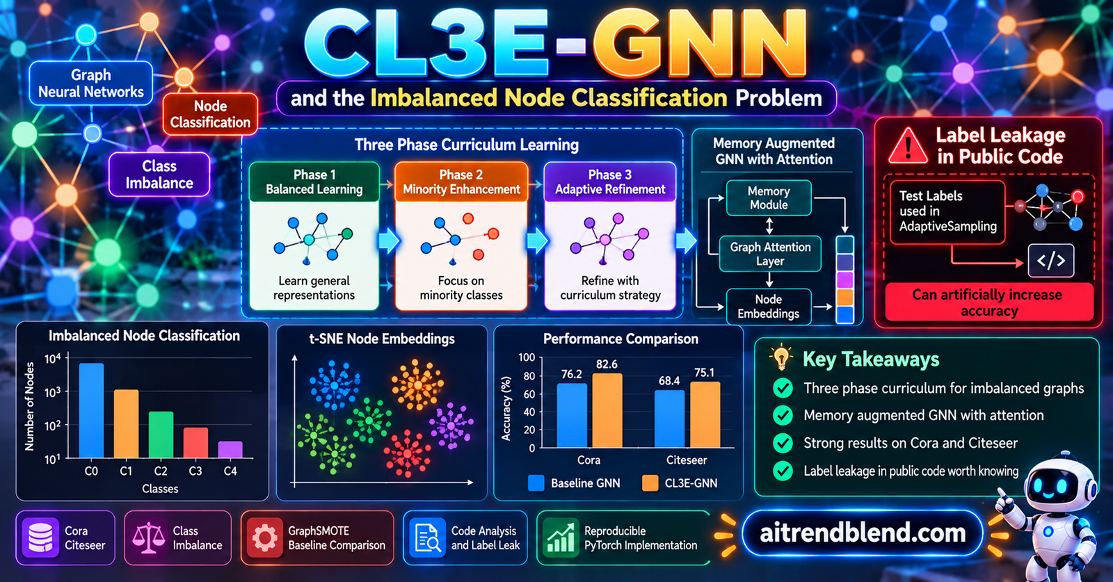
CL3E-GNN, from Abdul Joseph Fofanah, Lian Wen and David Chen at Griffith University with Shaoyang Zhang at Chang’an University and Alpha Alimamy Kamara at Central South University, takes on that problem with a curriculum borrowed from school teaching. Its three phases, called Engage, Enact and Embed, are meant to amplify minority signals early, refine them in the middle and lock them in at the end. The headline numbers are striking, including 96.1 percent accuracy on a heavily skewed version of Cora. We read the paper closely, opened the released code and ran a controlled experiment. What we found changes how those numbers should be read.
Key points
- CL3E-GNN stacks a GCN and GAT phase, an Enact phase with importance weights, two hop paths, uncertainty sampling, anomaly scores and edge intensity, and an Embed phase with memory and gradient based updates, all trained with a three stage curriculum loss.
- The paper reports large gains over 18 baseline variants on eight graphs, for example 96.1 percent accuracy on Cora against 83.5 percent for the best baseline.
- Its own backbone without any of the three phases scores 85.8 percent on Cora, above every baseline in the main table, which points to different training protocols rather than architecture alone.
- In the public code at commit 969c067, evaluation passes every node’s true label into the model, and one module scores each node, test nodes included, by distance to its own true class prototype.
- In our controlled test, that module alone raised a plain GCN’s test accuracy by 3.6 points on Cora and 6.5 points on Citeseer compared with the same module fed only training labels.
- Several reported standard deviations exceed what is mathematically possible for five runs of a metric between 0 and 1, and the full model’s Cora accuracy appears as five different values across the paper.
Why imbalance hurts graphs more than tables
Class imbalance is an old problem. In a spreadsheet, a minority row is still a row, and the usual fixes work on rows. You can duplicate it, interpolate new ones in the style of SMOTE, or give its errors a bigger weight in the loss. Each of those choices changes how much a rare example counts during training without touching what the example looks like.
Graphs break that tidy picture. A graph neural network builds each node’s representation from its neighbours. If a minority node sits among majority neighbours, its own features are blended with theirs at every layer. The authors put it well. Majority nodes dominate message passing and the aggregated information from minority nodes becomes statistically diluted. The minority class is not just rare in the loss. It is drowned out inside the features themselves.
That is why graph specific methods appeared. GraphSMOTE, from Zhao, Zhang and Wang, synthesises minority nodes in embedding space and trains an edge predictor to wire them into the graph. GraphMixup mixes minority embeddings with help from reinforcement learning. GraphSR augments data for the minority. ReVar, from Yan and colleagues, recasts the problem as a bias and variance trade off. LTE4G trains separate experts for head and tail classes. GATE-GNN, an earlier method by the same first author, combines several modules with spatial embeddings. Each tries to keep rare classes from vanishing during aggregation, either by adding nodes or by changing how examples are weighted.
CL3E-GNN’s angle is time. The authors argue that existing methods treat all training nodes uniformly or apply static reweighting that ignores how learning evolves. A curriculum, in the broad sense surveyed in IEEE TPAMI as a sequence of reweightings of the training distribution over time, can start with easy patterns and shift toward hard minority examples as the model improves.
Where the three phases come from
The phase names are taken from the Phases of Curriculum Implementation guidance published by the New South Wales Department of Education. Engage means exploring and planning change, Enact means teaching, assessing and refining, and Embed means consolidating practice. The paper maps these onto a network. Engage introduces simple node representations, Enact refines them with guided convolutions, and Embed consolidates them with memory. It also appeals to Vygotsky’s zone of proximal development and cites educational research suggesting that well sequenced instruction improves learning outcomes by 25 to 40 percent.
Analogies like this are helpful for explaining a design, and the paper is careful to say it presents the later phases using formal memory network and gradient formalisms rather than analogy. Still, it is worth keeping in mind that the educational evidence is about students, not gradient descent, and that the architecture should be judged on what each block computes. So let us look at exactly that.
How CL3E-GNN is built
Engage, two aggregators added together
The first phase runs a degree normalised graph convolution and a graph attention layer side by side on the same input, each with relational features \(F_{rn}\) added to the node features, and sums the results.
Here \(\zeta_\beta\) is a LeakyReLU with slope \(\beta\). The convolution provides a baseline of structural awareness even for isolated nodes, and the attention branch can, in principle, learn to up weight informative neighbours. Summing instead of concatenating keeps dimensions fixed.
Enact, many small tools in parallel
The second phase is the busiest. On top of its own convolution and attention, it computes three parallel attention maps, labelled structural, semantic and contextual, each with its own weight matrix, then a multi head version, and fuses them through a learned linear layer. Alongside that it runs six sub modules. Importance weights \(W_i = \sigma(W_w h_i + b_w)\) give each node a scalar. A metapath extractor summarises weighted multi hop paths. Adaptive sampling selects nodes that are uncertain or belong to minority classes. Edge intensity \(e_{ij} = \sigma(h_i^{\top}W_e h_j)\) scores each connection. Anomaly detection flags nodes far from their class prototype. A task embedding \(Z\) concatenates several of these outputs.
Read both definitions carefully, because they matter later. Minority membership \(v \in \mathcal{V}_{min}\) and the class prototype \(\mu_{c(v)}\) both need the node’s label \(c(v)\). For training nodes that is fine. For a test node, the label is exactly what the model is supposed to predict, so any use of it inside the forward pass has to be restricted to training nodes.
Embed, memory and gradient based updates
The third phase adds a differentiable memory matrix \(M\). Each node reads from it with softmax attention over memory slots, and the result is added to its representation.
Then five adaptation pathways are added on top. A cross task transfer \(W_{transfer} h_i^{source}\), a historical gradient step \(h_i + \gamma \nabla h_{prev}\), an error driven step \(h_i + \eta(y_{pred} – y_{true})\nabla_h \ell\), a context modulation \(h_i \odot c\), and a reward modulated step.
Again, \(y_{true}\) and \(y_i\) appear inside a representation update. During training on labelled nodes that is a legitimate design. At inference, the paper does not say how these terms are computed for unlabelled nodes. A faithful implementation should set them to zero there, and our reconstruction below does exactly that.
The outputs of all three phases are summed and passed through a two layer perceptron with a softmax.
A curriculum in the loss
The base loss is cross entropy with label smoothing. It is multiplied by a weight that changes with the training phase. During Engage the weight grows linearly with epochs. During Enact it grows for classes whose running accuracy lags the best class. During Embed it depends on how uncertain the prediction is.
with \(d_s = 1 – \max_c p(y=c\mid v)\). One detail is easy to miss. Since \(1 – d_s\) equals the model’s top probability, the Embed weight is largest for confident nodes, not uncertain ones. That is the opposite of what the paper’s prose describes as emphasising hard examples. It reads like an easy first weighting, which is closer to self paced learning than to hard example mining.
The danger in a model that reads labels inside its own forward pass is not that it is wrong to do so. It is that one unmasked line is enough to let the answer in. aitrendblend analysis of CL3E-GNN, Information Fusion 2027
What the experiments report
The evaluation covers eight graphs. Cora, Citeseer and PubMed are citation networks. Amazon Photo and Amazon Computers are co purchase graphs. Coauthor CS is a co authorship graph. Chameleon is a heterophilous Wikipedia graph, where linked pages tend to belong to different classes. OGBN-Arxiv, with 169,343 nodes and 1,166,243 edges, is the large scale test. Imbalance is created with a step protocol. Three classes are chosen at random as minorities and their sizes are reduced by a factor \(\Lambda\), up to \(\Lambda = 100\), where a minority class is about 1 percent of a majority class. Results are averaged over five runs, with paired t tests and bootstrap confidence intervals. The full results are in the CL3E-GNN paper in Information Fusion, which is open access.
| Method | Cora ACC | Cora F1 | Citeseer ACC | Citeseer F1 | PubMed ACC | PubMed F1 |
|---|---|---|---|---|---|---|
| Vanilla | 0.682 | 0.681 | 0.546 | 0.537 | 0.701 | 0.562 |
| GraphSMOTE | 0.747 | 0.743 | 0.575 | 0.567 | 0.757 | 0.635 |
| LTE4G | 0.828 | 0.810 | 0.702 | 0.657 | 0.848 | 0.842 |
| ReVar-GAT | 0.826 | 0.819 | 0.663 | 0.657 | 0.779 | 0.772 |
| GATE-GAT | 0.835 | 0.829 | 0.755 | 0.745 | 0.777 | 0.763 |
| Engage-GNN, phase one only | 0.937 | 0.929 | 0.902 | 0.898 | 0.872 | 0.862 |
| CL3E-GNN | 0.961 | 0.953 | 0.926 | 0.918 | 0.905 | 0.899 |
Table A. Selected rows from Table 5 of Fofanah et al., means over five runs. The paper lists 18 baseline rows in total, plus the three single phase variants.
On these numbers CL3E-GNN beats the best baseline by 12.6 points on Cora and 17.1 points on Citeseer. The other graphs show similar margins. Amazon Computers reaches 93.5 percent, Coauthor CS 96.5 percent, Chameleon 86.1 percent and OGBN-Arxiv 61.8 percent. A comparison against loss level fixes for imbalance on a GAT, using focal loss, class balanced loss and logit adjustment, shows those losses add 5.9 to 8.2 points over plain cross entropy while CL3E-GNN sits 20 points or more above them.
Here is where it gets interesting. Look at the Engage-GNN row. Phase one alone is a graph convolution and an attention layer summed together. That simple model scores 93.7 percent on Cora, more than ten points above every published method in the table, several of which are much more elaborate. And the ablation table goes further.
| Variant | What is active | Cora ACC | OGBN-Arxiv ACC |
|---|---|---|---|
| W/FE | GCN and GAT backbone features only | 0.858 | 0.532 |
| W/EW | Engage sub modules | 0.922 | 0.563 |
| W/2EW | Engage and Enact | 0.931 | 0.589 |
| W/3EW | All three phases, no curriculum | 0.949 | 0.602 |
| W/3EW CL | All three phases with curriculum | 0.950 | 0.615 |
| CL3E-GNN | Full model with feedback loops | 0.952 | 0.618 |
Table B. Component activation study from Table 12 of Fofanah et al.
The backbone variant W/FE, with none of the three phases, scores 85.8 percent on Cora. In Table A, the vanilla model scores 68.2 percent and the best published method 83.5 percent. In the loss comparison, a GAT trained with plain cross entropy also scores 68.2 percent. So the same kind of backbone appears at 68.2 percent in one table and 85.8 percent in another. The simplest explanation is that the baseline rows and the CL3E-GNN rows were not produced under the same conditions.
The paper says as much, in a sentence that is easy to skip. Different baselines may require different splits, and each baseline uses the split recommended by its original authors, while CL3E-GNN uses a fixed 70, 10, 20 split with seed 42. Many of the original imbalanced node classification papers use far fewer labelled nodes than 70 percent of the graph. A model trained on much more labelled data will score higher regardless of its architecture. The comparison in Table A therefore mixes two effects, method and supervision, and cannot separate them.
The ablation table is the most informative comparison in the paper, because every row uses the same code and split. Within it, the three phases add about 9.4 points on Cora and 8.6 points on OGBN-Arxiv over the backbone. The much larger gaps against published baselines mix in differences of protocol.
One model, five accuracies on Cora
Reading across the paper, the full model’s Cora accuracy at the most severe imbalance appears in several places, and the values do not agree.
| Where it appears | Setting stated | Reported Cora accuracy |
|---|---|---|
| Table 5, main results | Step imbalance | 0.961 |
| Tables 6 and 13, loss comparison | \(\Lambda = 100\) | 0.961 |
| Table 12, component study | Not stated | 0.952 |
| Table 11, feature ablation | Not stated | 0.950 |
| Section 6.4.1 text | \(\Lambda = 100\) | 0.892 |
| Table 10, label scarcity | \(\Lambda = 0.1\) | 0.997 |
Table C. Full model Cora accuracy across the paper, compiled by the aitrendblend team.
Part of this is a notation problem. The symbol \(\Lambda\) means a downsampling factor between 10 and 100 in Section 6.1 and a fraction of labelled minority nodes between 0.1 and 0.8 in Section 6.5.2. Still, the same setting, \(\Lambda = 100\), gives 0.961 in two tables and 0.892 in the text. And at a 10 percent labelled fraction, Table 10 reports 99.7 percent accuracy on Cora and 99.3 percent on Citeseer, higher than the main results with more labels. For context, in our own runs below a plain GCN trained on 60 percent of balanced Citeseer reaches about 77 percent.
Standard deviations that cannot happen
Accuracy, AUC and F1 all lie between 0 and 1. For five runs of such a metric, the largest possible sample standard deviation is about 0.55, reached only when two or three runs score exactly 0 and the rest score exactly 1. Table 8 reports LTE4G on OGBN-Arxiv at an accuracy of 0.526 ± 1.521 and an AUC of 0.678 ± 1.521, and LTE4G on Amazon Photo at an accuracy of 0.915 ± 0.811 and an F1 of 0.901 ± 0.801. These values cannot be standard deviations of the stated metrics. They may be typographical errors, or a different statistic, but as printed they cannot be checked against anything. Several other baseline entries, such as a ReVar-GCN Cora accuracy of 0.819 ± 0.222, are possible only if one run collapsed badly, which would deserve comment.
What we found in the released code
The authors deserve credit for publishing their code, which is what made this check possible. We inspected the public CL3E-GNN repository at commit 969c067, dated 6 September 2026. We read the code. We did not run the repository itself.
Three things stand out. First, every evaluation path, in both the training script and the main entry point, calls the model with the full label vector and the training mask, in the form partial_labels=data.y, mask=data.train_mask. The labels of validation and test nodes are therefore inside the forward pass at evaluation time.
Second, most modules that read labels respect the mask. The importance prototypes, the anomaly scores and the reward signal only use labelled training nodes. The adaptive sampling module does not. It builds class prototypes from training nodes, which is fine, but then computes for every node in the graph the distance to the prototype of that node’s own true class, divided by the distance to the nearest other prototype, and uses that ratio to scale the node’s features. For a test node, this ratio is small when the node really belongs to the class its label says, so the scaling carries information about the answer.
Third, we could not find code in the repository that applies the step imbalance protocol. The data loader creates a random split of 60, 20 and 20 percent, not the 70, 10 and 20 stated in the paper, and does not downsample minority classes. The paper’s experiments may have used other scripts that are not in the repository.
How much does the leak matter
Reading code only tells you a leak is possible. To see whether it matters, we built the smallest experiment we could. We took a standard two layer GCN and added the sampling block with the same scoring rule as the released code, then trained three versions on Cora and Citeseer with random 60, 20 and 20 splits, keeping the test accuracy at the epoch of best validation accuracy, over five seeds. The plain GCN has no sampling block. The honest version passes the block training labels only, with every other label hidden. The leaky version passes all labels with the training mask, exactly as the released evaluation code does.
| Model | Labels visible to the forward pass | Cora test accuracy | Citeseer test accuracy |
|---|---|---|---|
| Plain two layer GCN | None | 0.874 ± 0.009 | 0.769 ± 0.004 |
| GCN plus sampling block, honest | Training nodes only | 0.880 ± 0.014 | 0.762 ± 0.011 |
| GCN plus sampling block, as released | All nodes, with training mask | 0.917 ± 0.010 | 0.827 ± 0.005 |
Table D. Our own controlled experiment, five seeds each, balanced classes, no imbalance protocol. Cora ran for 200 epochs and Citeseer for 120. The script is included below.
The honest block does essentially nothing. The leaky block adds 3.6 points on Cora and 6.5 points on Citeseer, without any change to architecture or training other than which labels the block can see. That is a single module inside a much larger model. In the full CL3E-GNN, the leaked score feeds the task embedding and the fusion, and the effect could be larger or smaller.
We want to be precise about what this does and does not show. It shows that the released code, as written, lets test labels influence test predictions, and that this kind of influence is large enough to matter on the same benchmarks. It does not show which code produced the numbers in the paper, and it does not explain the protocol differences discussed above on its own. The right next step is for the authors to rerun evaluation with all non training labels hidden and report the result. If the numbers hold, the method stands on firmer ground. If they drop, the field learns something useful about where the gains came from.
Any graph model that reads labels inside its forward pass should be evaluated with every non training label replaced by a placeholder. It is a one line change, and it removes the question entirely.
What the theory does and does not say
The paper presents six theorems and six corollaries, covering gradient stability, risk decomposition, memory convergence, a reward term, global convergence and complexity. Proofs are in the appendix. A full review of them is beyond this article, but three observations matter for readers deciding how much weight to give them.
The imbalance model differs from the experiments. The theory assumes class probabilities fall exponentially, \(P(y=c) \propto e^{-\lambda c}\), so every class is smaller than the one before. The experiments use a step protocol, with majority classes untouched and three minorities shrunk by the same factor. Bounds derived under one distribution do not automatically transfer to the other.
The imbalance penalty shrinks as imbalance grows. Theorem 1 bounds the Engage gradient by three terms, the last of which is \(\lambda e^{-\lambda} L\).
That term peaks at \(\lambda = 1\) with a value of about 0.37 L and falls to about 0.15 L at \(\lambda = 3\) and 0.03 L at \(\lambda = 5\). Read literally, the bound says extreme imbalance makes gradients more stable than mild imbalance, and Corollary 1 accordingly recommends a shorter warmup for more imbalanced data. Either the bound captures something counterintuitive that needs explaining, or the penalty term should grow with imbalance.
Adding a term does not improve a bound. Theorem 4 adds a \(\rho^2\) term for the reward signal and describes it as improving the convergence bound. Adding a positive term to an upper bound loosens it. The reward update may still help in practice, but the theorem as stated shows a cost, not a benefit.
None of this makes the theory useless. Bounds of this form can guide hyperparameter choices, and the paper’s empirical plots of gradient norms and loss curves are informative. But the guarantees describe a simplified model, and should be read as motivation rather than as proof that the architecture works.
Cost and complexity
CL3E-GNN has 378 thousand parameters on Cora and 523 thousand on Citeseer, far fewer than GATE-GNN’s 4.5 million and 28.4 million but more than ReVar’s 96 thousand and 242 thousand. Inference costs 1.02 GFLOPs on Cora and 1.71 on Citeseer. Each layer runs four GAT level attention operations against one in a plain GAT, and the authors report training time 30 to 45 percent above a GAT baseline, with an average runtime of 4.2 hours per dataset on a T4 GPU. Per epoch complexity is \(O(|\mathcal{E}|H + NH^2 + NC + |\mathcal{E}|L_{path})\), dominated by \(NH^2\), which is in line with standard graph networks.
The loss ablation on OGBN-Arxiv has a twist. The best configuration, at 61.8 percent accuracy, uses time based and difficulty based weighting without standard cross entropy. Adding standard cross entropy back lowers accuracy to 57.4 percent. The class performance weighting that defines the Enact phase of the loss is not tested separately at all. The abstract describes a dual loss combining cross entropy with the curriculum term, so it is unclear which configuration the headline numbers use.
Where CL3E-GNN fits
The ideas inside CL3E-GNN are reasonable, and several have a track record elsewhere. Adding a convolution and an attention aggregator is a cheap way to combine structure and selectivity. Uncertainty driven sampling and prototype based anomaly scores are standard tools, and memory modules have helped models retain rare patterns in other domains. Our earlier piece on HPGRL’s hierarchical prototypes for graph classification shows how prototypes can make graph models resist noise, and our explainer on the mathematics of graph neural networks covers why neighbourhood averaging smooths minority signals in the first place.
The difficulty is in how many of these tools are stacked at once. With a dozen interacting blocks, attributing a gain to any one of them is hard, and the curriculum story, while appealing, is not tested in a way that separates it from the extra capacity it comes with. The cleanest evidence for the curriculum itself is the small step from W/3EW to W/3EW CL in Table B, 0.1 points on Cora and 1.3 points on OGBN-Arxiv.
For practitioners, the lesson is about evaluation as much as architecture. Transductive node classification, where the model sees the whole graph including unlabelled nodes during training, makes it unusually easy for label information to slip through. Methods like label propagation, which we discussed in our analysis of MIFOMO, use labels by design and are careful to restrict them to the support set. Any architecture that computes prototypes, rewards or class memberships inside the forward pass needs the same discipline.
Limitations
Comparability. Baselines were run on splits recommended by their original papers, while CL3E-GNN used a fixed 70, 10, 20 split. The gap between the paper’s own backbone at 85.8 percent and the vanilla baseline at 68.2 percent on Cora suggests the protocols differ substantially.
Reproducibility. The public code passes all labels into the forward pass at evaluation, and one module uses them for test nodes. We could not find the step imbalance protocol in the repository, and the default split differs from the paper.
Internal consistency. The full model’s Cora accuracy appears as 0.892, 0.950, 0.952, 0.961 and 0.997 in different places. The symbol \(\Lambda\) has two meanings. Several standard deviations exceed the mathematical maximum for the reported metrics. The introduction mentions seven datasets while the experiments use eight.
Single seed splits. All runs use seed 42 for the split, so the five repetitions vary initialisation, not which nodes are labelled. Variation across splits, often larger for small graphs like Cora and Citeseer, is not measured.
Theory and practice. The theoretical imbalance model differs from the experimental protocol, the Theorem 1 penalty decreases with imbalance, and Theorem 4 describes a looser bound as an improvement.
Scope. All graphs are standard academic benchmarks with induced imbalance. No naturally imbalanced graph, such as a real fraud or rare disease network, is tested, although the paper names these as applications.
Reproducing CL3E-GNN in PyTorch
The first listing below is our independent reconstruction of CL3E-GNN from the paper’s equations, in plain PyTorch with no graph library. It includes the dual GCN and GAT Engage phase, an Enact phase with the three attention maps, multi head attention, importance weights, two hop paths, uncertainty and minority sampling, prototype anomaly scores, edge intensity and the task embedding, an Embed phase with memory read, transfer, historical gradient, error feedback, context and reward pathways, the three stage curriculum loss, the step imbalance protocol and the four metrics.
One choice is deliberate. Every module that reads labels receives a label vector in which all non training labels are replaced by a placeholder, and minority membership, prototypes, error feedback and rewards are computed for training nodes only. On a synthetic graph with three minority classes kept at 4 training nodes each, it reaches 92.8 percent test accuracy and 92.3 percent balanced accuracy, about one point above a plain GCN at 91.7 and 91.2 on the same split. That modest margin is what we would expect from an honest implementation on an easy synthetic task.
# CL3E-GNN reference implementation (aitrendblend reconstruction)
# Based on Fofanah, Wen, Chen, Zhang and Kamara, "CL3E-GNN, three phase attention with feature
# fusion based on curriculum implementation strategy for class imbalanced node classification",
# Information Fusion 138 (2027) 104745. Official code: https://github.com/afofanah/CL3E-GNN
#
# Independent reconstruction from the paper's equations, written in plain PyTorch.
# One deliberate difference from the released code: every module that reads labels sees ONLY
# training labels. Labels of validation and test nodes are never passed into the forward pass.

import math
import torch
import torch.nn as nn
import torch.nn.functional as F


# ---------------------------------------------------------------------------
# 0. Graph helpers (edge list form, self loops added once)
# ---------------------------------------------------------------------------
def add_self_loops(ei, n):
    loops = torch.arange(n).repeat(2, 1)
    return torch.cat([ei, loops], 1)


def scatter_sum(src, index, n):
    out = torch.zeros(n, *src.shape[1:], dtype=src.dtype)
    return out.index_add_(0, index, src)


def scatter_mean(src, index, n):
    cnt = scatter_sum(torch.ones(len(index), 1), index, n).clamp_min(1)
    return scatter_sum(src, index, n) / cnt


def edge_softmax(scores, dst, n):
    """Softmax of edge scores over the incoming edges of each destination node."""
    m = torch.full((n,), -1e9).scatter_reduce(0, dst, scores, "amax", include_self=True)
    e = torch.exp(scores - m[dst])
    return e / scatter_sum(e, dst, n)[dst].clamp_min(1e-16)


class GCNLayer(nn.Module):
    """Degree normalised convolution, Eq. 13, 17 and 33."""
    def __init__(self, i, o):
        super().__init__()
        self.W = nn.Linear(i, o)

    def forward(self, h, ei):
        src, dst = ei
        deg = scatter_sum(torch.ones(src.size(0)), dst, h.size(0))
        norm = (deg[src] * deg[dst]).rsqrt()
        return scatter_sum(self.W(h)[src] * norm[:, None], dst, h.size(0))


class GATLayer(nn.Module):
    """Single head additive attention with LeakyReLU slope beta, Eq. 14."""
    def __init__(self, i, o, beta=0.2):
        super().__init__()
        self.W = nn.Linear(i, o, bias=False)
        self.a = nn.Parameter(torch.randn(2 * o) * 0.1)
        self.beta = beta

    def coeffs(self, h, ei):
        src, dst = ei
        z = self.W(h)
        s = F.leaky_relu(torch.cat([z[dst], z[src]], 1) @ self.a, self.beta)
        return edge_softmax(s, dst, h.size(0)), z

    def forward(self, h, ei):
        alpha, z = self.coeffs(h, ei)
        return scatter_sum(alpha[:, None] * z[ei[0]], ei[1], h.size(0))


# ---------------------------------------------------------------------------
# 1. Engage phase, dual GCN and GAT aggregation summed (Eq. 13 to 16)
# ---------------------------------------------------------------------------
class Engage(nn.Module):
    def __init__(self, d_in, h):
        super().__init__()
        self.rel = nn.Linear(d_in, d_in, bias=False)        # relational features F_rn
        self.gcn, self.gat = GCNLayer(d_in, h), GATLayer(d_in, h)

    def forward(self, x, ei):
        src, dst = ei
        x_rel = x + self.rel(scatter_mean(x[src], dst, x.size(0)))   # h tilde = h + F_rn
        return F.relu(self.gcn(x_rel, ei)) + F.relu(self.gat(x_rel, ei))


# ---------------------------------------------------------------------------
# 2. Three attention maps fused (Eq. 19 to 22), shared by Enact and Embed
# ---------------------------------------------------------------------------
class TripleAttention(nn.Module):
    def __init__(self, h, heads=4):
        super().__init__()
        self.gat = GATLayer(h, h)
        self.Ws = nn.ModuleList([nn.Linear(h, h, bias=False) for _ in range(3)])  # struct, sem, ctx
        self.heads = nn.ModuleList([GATLayer(h, h // heads) for _ in range(heads)])
        self.fuse = nn.Linear(3 * h + h, h)

    def forward(self, H, ei):
        alpha, _ = self.gat.coeffs(H, ei)
        src, dst = ei
        maps = [scatter_sum(alpha[:, None] * W(H)[src], dst, H.size(0)) for W in self.Ws]
        multi = torch.cat([F.elu(hd(H, ei)) for hd in self.heads], 1)                # Eq. 20
        return self.fuse(torch.cat(maps + [multi], 1))


# ---------------------------------------------------------------------------
# 3. Enact phase (Eq. 23 to 31), labels restricted to the training mask
# ---------------------------------------------------------------------------
class Enact(nn.Module):
    def __init__(self, h, n_classes, tau_uncert=0.5, lambda_ano=2.0):
        super().__init__()
        self.C, self.tau, self.lam = n_classes, tau_uncert, lambda_ano
        self.gcn, self.att = GCNLayer(h, h), TripleAttention(h)
        self.Ww = nn.Linear(h, 1)                         # importance weights, Eq. 23
        self.meta = nn.Linear(h, h)                       # two hop metapath summary, Eq. 24 and 25
        self.We = nn.Linear(h, h, bias=False)             # edge intensity, Eq. 27
        self.Wz = nn.Linear(4 * h, h)                     # task embedding Z, Eq. 29
        self.probe = nn.Linear(h, n_classes)              # uncertainty for sampling, Eq. 26

    def forward(self, H, ei, y_train, train_mask):
        n, (src, dst) = H.size(0), ei
        W_imp = torch.sigmoid(self.Ww(H)).squeeze(1)                                  # Eq. 23
        h1 = scatter_mean(H[src], dst, n)
        F_weight = self.meta(scatter_mean(h1[src], dst, n))                          # 2 hop paths
        # Adaptive sampling, Eq. 26. Uncertainty comes from predictions, minority membership
        # only from training labels. Nodes outside the training set use predictions only.
        p = torch.softmax(self.probe(H), 1)
        uncertain = (1 - p.max(1).values) > self.tau
        counts = torch.bincount(y_train[train_mask], minlength=self.C).float()
        minority_cls = counts < counts[counts > 0].median()
        is_min = torch.zeros(n, dtype=torch.bool)
        is_min[train_mask] = minority_cls[y_train[train_mask]]
        S = (uncertain | is_min).float()
        # Anomaly detection, Eq. 28, prototypes and deviations from training nodes only
        A = torch.zeros(n)
        for c in range(self.C):
            cm = train_mask & (y_train == c)
            if cm.sum() > 1:
                mu = H[cm].mean(0)
                dist = (H[cm] - mu).norm(dim=1)
                A[cm] = (dist > self.lam * dist.std()).float()
        # Edge intensity, Eq. 27, applied as (E ⊙ A) H
        e = torch.sigmoid((self.We(H[src]) * H[dst]).sum(1))
        edge_term = scatter_sum(e[:, None] * H[src], dst, n)
        gcn_out, att_out = self.gcn(H, ei), self.att(H, ei)
        Z = self.Wz(torch.cat([H, F_weight, gcn_out, att_out], 1))                    # Eq. 29
        Z = Z * (1 + 0.5 * S - 0.5 * A)[:, None]          # sampled nodes up, anomalies down
        return F.relu(gcn_out) + att_out + W_imp[:, None] * Z + edge_term             # Eq. 30 and 31


# ---------------------------------------------------------------------------
# 4. Embed phase (Eq. 39 to 48, Algorithms 1 and 2), training labels only
# ---------------------------------------------------------------------------
class Embed(nn.Module):
    def __init__(self, h, n_classes, slots=None, tau_mem=1.0, gamma=0.1, eta=0.1, rho=0.1,
                 g_max=1.0):
        super().__init__()
        self.gcn, self.att = GCNLayer(h, h), TripleAttention(h)
        self.M = nn.Parameter(torch.randn(h, slots or h) * 0.1)                       # memory
        self.W_transfer = nn.Linear(h, h, bias=False)
        self.c = nn.Parameter(torch.ones(h))                                          # context
        self.head = nn.Linear(h, n_classes)               # gives the loss gradient w.r.t. h
        self.tau_mem, self.gamma, self.eta, self.rho, self.g_max = tau_mem, gamma, eta, rho, g_max
        self.register_buffer("g_prev", torch.zeros(1))
        self.register_buffer("pred_prev", torch.zeros(1, dtype=torch.long))

    def forward(self, H, ei, y_train, train_mask, source=None):
        n = H.size(0)
        w = torch.softmax(H @ self.M / self.tau_mem, 1)                                # Algorithm 1
        h_m = H + w @ self.M.t()                                                      # Eq. 39
        h_t = self.W_transfer(source if source is not None else H)                   # transfer
        g = self.g_prev if self.g_prev.numel() == H.numel() else torch.zeros_like(H)
        h_h = H + self.gamma * g.view_as(H).clamp(-self.g_max, self.g_max)            # history
        h_c = H * self.c                                                              # context
        # Error driven feedback and reward update use dl/dh = (p - y) W for training nodes only
        logits = self.head(H)
        p = torch.softmax(logits, 1)
        y1h = torch.zeros_like(p)
        y1h[train_mask] = F.one_hot(y_train[train_mask], p.size(1)).float()
        grad_h = ((p - y1h) * train_mask[:, None].float()) @ self.head.weight         # dl/dh
        h_f = H - self.eta * grad_h                     # step against the error, Eq. 41 row 3
        pred = logits.argmax(1)
        r = torch.zeros(n)
        if self.pred_prev.numel() == n:
            now = (pred == y_train) & train_mask
            before = (self.pred_prev == y_train) & train_mask
            r = now.float() - before.float()                                          # Eq. 42
        h_r = H + self.rho * r[:, None] * grad_h                                      # Eq. 43
        if self.training:
            self.pred_prev = pred.detach()
            self.g_prev = grad_h.detach()
        return (F.relu(self.gcn(H, ei)) + self.att(H, ei) + h_m + h_t + h_h + h_f + h_c + h_r)


# ---------------------------------------------------------------------------
# 5. Full model, phase outputs summed then a two layer MLP (Eq. 49 and 50)
# ---------------------------------------------------------------------------
class CL3EGNN(nn.Module):
    def __init__(self, d_in, h, n_classes, dropout=0.5):
        super().__init__()
        self.engage = Engage(d_in, h)
        self.enact = Enact(h, n_classes)
        self.embed = Embed(h, n_classes)
        self.norm = nn.ModuleList([nn.LayerNorm(h) for _ in range(3)])
        self.mlp = nn.Sequential(nn.Linear(h, h), nn.ReLU(), nn.Dropout(dropout), nn.Linear(h, n_classes))
        self.drop = dropout

    def forward(self, x, ei, y_train, train_mask):
        x = F.dropout(x, self.drop, self.training)
        H_E = self.norm[0](self.engage(x, ei))
        H_A = self.norm[1](self.enact(H_E, ei, y_train, train_mask))
        H_B = self.norm[2](self.embed(H_A, ei, y_train, train_mask, source=H_E))
        return self.mlp(F.dropout(H_E + H_A + H_B, self.drop, self.training))


# ---------------------------------------------------------------------------
# 6. Curriculum loss with three weighting regimes (Eq. 51 to 56)
# ---------------------------------------------------------------------------
class CurriculumLoss:
    def __init__(self, n_classes, e_warmup=20, e1=30, e2=60, w_init=0.3, w_final=1.0,
                 smooth=0.1, momentum=0.9):
        self.C, self.ew, self.e1, self.e2 = n_classes, e_warmup, e1, e2
        self.wi, self.wf, self.s, self.m = w_init, w_final, smooth, momentum
        self.A = torch.full((n_classes,), 1.0 / n_classes)        # running class accuracy

    def w_t(self, e):
        return self.wi + (self.wf - self.wi) * min(1.0, e / self.ew)                  # Eq. 52

    def __call__(self, logits, y, e):
        base = F.cross_entropy(logits, y, label_smoothing=self.s, reduction="none")   # Eq. 51
        p = torch.softmax(logits.detach(), 1)
        acc = torch.stack([(p.argmax(1)[y == c] == c).float().mean() if (y == c).any()
                           else self.A[c] for c in range(self.C)])
        self.A = self.m * self.A + (1 - self.m) * acc
        wt = self.w_t(e)
        if e < self.e1:
            w = torch.full_like(base, wt)                                             # Engage
        elif e < self.e2:
            w = wt + (1 - wt) * (1 - self.A[y] / self.A.max().clamp_min(1e-8))       # Eq. 53
        else:
            d = 1 - p.max(1).values                                                   # difficulty
            w = wt + (1 - wt) * (1 - d)                                               # Eq. 54
        return (w * base).mean()


# ---------------------------------------------------------------------------
# 7. Step imbalance protocol and metrics
# ---------------------------------------------------------------------------
def step_imbalance_split(y, n_minority=3, lam=10, frac=(0.6, 0.2), seed=0):
    """Random split, then keep only 1/lam of the training nodes of n_minority random classes."""
    g = torch.Generator().manual_seed(seed)
    n, C = len(y), int(y.max()) + 1
    perm = torch.randperm(n, generator=g)
    a, b = int(frac[0] * n), int((frac[0] + frac[1]) * n)
    tr, va, te = [torch.zeros(n, dtype=torch.bool) for _ in range(3)]
    tr[perm[:a]], va[perm[a:b]], te[perm[b:]] = True, True, True
    minority = torch.randperm(C, generator=g)[:n_minority]
    for c in minority.tolist():
        idx = torch.nonzero(tr & (y == c)).squeeze(1)
        keep = max(1, len(idx) // lam)
        tr[idx[keep:]] = False
    return tr, va, te, minority


def metrics(logits, y, mask, C):
    p = torch.softmax(logits[mask], 1); t = y[mask]; pred = p.argmax(1)
    acc = (pred == t).float().mean().item()
    rec, f1s, aucs = [], [], []
    for c in range(C):
        tp = ((pred == c) & (t == c)).sum().item(); fn = ((pred != c) & (t == c)).sum().item()
        fp = ((pred == c) & (t != c)).sum().item()
        if tp + fn == 0:
            continue
        r = tp / (tp + fn); pr = tp / (tp + fp) if tp + fp else 0.0
        rec.append(r); f1s.append(2 * pr * r / (pr + r) if pr + r else 0.0)
        s = p[:, c]; pos = t == c
        if 0 < pos.sum() < len(t):
            rk = torch.empty_like(s); rk[s.argsort()] = torch.arange(1, len(s) + 1).float()
            n1, n0 = pos.sum().item(), (~pos).sum().item()
            aucs.append(((rk[pos].sum() - n1 * (n1 + 1) / 2) / (n1 * n0)).item())
    return {"ACC": acc, "bAcc": sum(rec) / len(rec), "F1": sum(f1s) / len(f1s),
            "AUC": sum(aucs) / len(aucs)}


# ---------------------------------------------------------------------------
# 8. Training loop
# ---------------------------------------------------------------------------
def train(model, x, ei, y, tr, va, epochs=90, lr=0.005, wd=5e-4):
    C = int(y.max()) + 1
    y_train = torch.where(tr, y, torch.zeros_like(y))        # hide every non training label
    crit = CurriculumLoss(C)
    opt = torch.optim.Adam(model.parameters(), lr=lr, weight_decay=wd)
    best, state = -1.0, None
    for e in range(epochs):
        model.train(); opt.zero_grad()
        loss = crit(model(x, ei, y_train, tr)[tr], y[tr], e)
        loss.backward(); opt.step()
        model.eval()
        with torch.no_grad():
            m = metrics(model(x, ei, y_train, tr), y, va, C)
        if m["bAcc"] > best:
            best, state = m["bAcc"], {k: v.clone() for k, v in model.state_dict().items()}
    model.load_state_dict(state)
    return model, y_train


# ---------------------------------------------------------------------------
# 9. Smoke test on a synthetic stochastic block graph with three minority classes
# ---------------------------------------------------------------------------
if __name__ == "__main__":
    torch.manual_seed(0)
    C, per, d = 6, 150, 32
    y = torch.arange(C).repeat_interleave(per)
    n = len(y)
    centers = torch.randn(C, d)
    x = centers[y] * 0.6 + torch.randn(n, d)
    same = (y[:, None] == y[None, :])
    prob = torch.where(same, torch.tensor(0.04), torch.tensor(0.004))
    adj = torch.triu(torch.rand(n, n) < prob, 1)
    ei = torch.nonzero(adj | adj.t()).t()
    ei = add_self_loops(ei, n)
    tr, va, te, minority = step_imbalance_split(y, lam=20, seed=1)
    print("minority classes:", minority.tolist(),
          " training nodes per class:", torch.bincount(y[tr], minlength=C).tolist())

    model = CL3EGNN(d, 64, C)
    print("parameters:", sum(p.numel() for p in model.parameters()))
    model, y_train = train(model, x, ei, y, tr, va)
    model.eval()
    with torch.no_grad():
        out = model(x, ei, y_train, tr)
    print("CL3E-GNN test:", {k: round(v, 3) for k, v in metrics(out, y, te, C).items()})

    # Plain two layer GCN on the same split, for reference
    class GCN(nn.Module):
        def __init__(s):
            super().__init__(); s.l1, s.l2 = GCNLayer(d, 64), GCNLayer(64, C)
        def forward(s, x, ei, *_):
            return s.l2(F.dropout(F.relu(s.l1(F.dropout(x, 0.5, s.training), ei)), 0.5, s.training), ei)
    g = GCN(); opt = torch.optim.Adam(g.parameters(), lr=0.01, weight_decay=5e-4)
    best, st = -1, None
    for e in range(150):
        g.train(); opt.zero_grad(); F.cross_entropy(g(x, ei)[tr], y[tr]).backward(); opt.step()
        g.eval()
        with torch.no_grad():
            b = metrics(g(x, ei), y, va, C)["bAcc"]
        if b > best:
            best, st = b, {k: v.clone() for k, v in g.state_dict().items()}
    g.load_state_dict(st); g.eval()
    with torch.no_grad():
        print("Plain GCN test:", {k: round(v, 3) for k, v in metrics(g(x, ei), y, te, C).items()})
The second listing is the leakage check behind Table D. It uses PyTorch Geometric to load Cora and Citeseer, and reproduces the released sampling rule in a few lines. Running it with all labels and with training labels only is enough to see the difference.
# Leakage check for the AdaptiveSampling score used in the public CL3E-GNN code.
# Compares a plain 2 layer GCN with the same GCN plus a sampling block that is fed
# (a) all labels with a train mask, as in the released evaluation code, and
# (b) only training labels, with every other label hidden.
import sys
import torch
import torch.nn as nn
import torch.nn.functional as F
from torch_geometric.datasets import Planetoid
from torch_geometric.nn import GCNConv
from torch_geometric.utils import degree, scatter

root = sys.argv[1]
ds_name = sys.argv[2] if len(sys.argv) > 2 else "Cora"
data = Planetoid(root, ds_name)[0]
N, C = data.num_nodes, int(data.y.max()) + 1


def split(seed, tr=0.6, va=0.2):
    g = torch.Generator().manual_seed(seed)
    p = torch.randperm(N, generator=g)
    a, b = int(N * tr), int(N * (tr + va))
    m = lambda idx: torch.zeros(N, dtype=torch.bool).index_fill_(0, idx, True)
    return m(p[:a]), m(p[a:b]), m(p[b:])


class Sampling(nn.Module):
    """Same scoring rule as AdaptiveSampling in the released code."""
    def __init__(self, h):
        super().__init__()
        self.t = nn.Sequential(nn.Linear(h, h), nn.LayerNorm(h), nn.GELU())
        self.o = nn.Sequential(nn.Linear(h, h), nn.LayerNorm(h), nn.GELU())

    def forward(self, x, ei, labels, mask):
        src, dst = ei
        nd = degree(src, x.size(0)); nd = nd / (nd.max() + 1e-8)
        pr = torch.stack([x[mask][labels[mask] == c].mean(0) for c in range(C)])
        d = torch.cdist(x, pr)
        lab = labels.clamp(min=0)
        od = d[torch.arange(x.size(0)), lab]
        im = torch.zeros_like(d).scatter_(1, lab.unsqueeze(1), float("inf"))
        sc = 0.5 * od / ((d + im).min(1).values + 1e-8) + 0.3 * nd + 0.2 * (1 - mask.float())
        t = self.t(x) * sc.unsqueeze(1)
        return self.o(0.7 * t + 0.3 * scatter(t[src], dst, 0, dim_size=x.size(0), reduce="mean"))


class Net(nn.Module):
    def __init__(self, use_sampling, h=64):
        super().__init__()
        self.c1, self.c2 = GCNConv(data.num_features, h), GCNConv(h, h)
        self.s = Sampling(h) if use_sampling else None
        self.cls = nn.Linear(h, C)

    def forward(self, x, ei, labels, mask):
        h = F.dropout(F.relu(self.c1(F.dropout(x, 0.5, self.training), ei)), 0.5, self.training)
        h = F.relu(self.c2(h, ei))
        if self.s is not None:
            h = h + self.s(h, ei, labels, mask)
        return self.cls(h)


def run(mode, seed):
    torch.manual_seed(seed)
    tr, va, te = split(seed)
    if mode == "leaky":            # labels of every node visible, as in the released code
        labels = data.y
    else:                          # honest: non training labels replaced by a dummy value
        labels = torch.where(tr, data.y, torch.zeros_like(data.y))
    m = Net(mode != "gcn")
    opt = torch.optim.Adam(m.parameters(), lr=0.01, weight_decay=5e-4)
    best_va, best_te = 0, 0
    for ep in range(int(sys.argv[3]) if len(sys.argv) > 3 else 200):
        m.train(); opt.zero_grad()
        F.cross_entropy(m(data.x, data.edge_index, labels, tr)[tr], data.y[tr]).backward(); opt.step()
        m.eval()
        with torch.no_grad():
            p = m(data.x, data.edge_index, labels, tr).argmax(1)
        a_va = (p[va] == data.y[va]).float().mean().item()
        a_te = (p[te] == data.y[te]).float().mean().item()
        if a_va > best_va:
            best_va, best_te = a_va, a_te
    return best_te


for mode in ["gcn", "honest", "leaky"]:
    accs = torch.tensor([run(mode, s) for s in range(5)])
    print(f"{ds_name:9s} {mode:7s} test acc {accs.mean():.4f} +- {accs.std():.4f}")
What CL3E-GNN leaves for the field
CL3E-GNN sets out to solve a real and stubborn problem. Graph neural networks average away rare classes, and the paper’s answer is to give learning a schedule, amplifying minority signals early, refining them with targeted tools and preserving them with memory. The design is thoughtful, the code is public and the evaluation spans eight graphs, which is more than many papers in this area attempt.
The conceptual contribution worth keeping is the idea that imbalance remedies should change over training rather than stay fixed. Static reweighting treats a minority node the same in the first epoch as in the last, even though what the model needs from it changes. A schedule that moves from stabilising to targeting to consolidating is a sensible hypothesis, and the internal ablation gives it modest support.
That idea transfers well beyond citation graphs. Fraud rings, rare disease patients in clinical knowledge graphs and attack traffic in network logs all have the same structure, a small class embedded among a large one. A phased curriculum could be combined with any backbone, including the leaner ones, and tested on graphs where imbalance occurs naturally rather than being induced.
The headline results, though, cannot yet be taken at face value. The baselines and the proposed model appear to have been trained under different protocols, the paper reports inconsistent values for its own model, some reported variances are impossible, and the public code lets test labels into the forward pass through a module whose leak alone is worth several points on the same benchmarks in our test.
The fix is straightforward and the authors are well placed to make it. Hide every non training label at evaluation, run all methods on the same splits with several split seeds, and report the result. If CL3E-GNN keeps a clear lead under those conditions, it will be a stronger paper and a more useful tool. Either way, the episode is a reminder that in transductive graph learning, the most important line of code is often the one that decides which labels the model is allowed to see.
Frequently asked questions
What is CL3E-GNN?
CL3E-GNN is a graph neural network for node classification when some classes are very rare. It trains in three phases called Engage, Enact and Embed, combining graph convolution and attention, sampling and anomaly tools, a memory module and a curriculum loss that changes its weighting as training progresses.
Why is class imbalance harder on graphs?
A graph neural network builds each node’s representation by averaging its neighbours. When a rare class node is surrounded by common class neighbours, its own signal is blended away at every layer, so the problem affects the features themselves and not only the loss.
What accuracy does CL3E-GNN report?
The paper reports 96.1 percent accuracy on Cora and 92.6 percent on Citeseer under heavy imbalance, with the best baselines at 83.5 and 75.5 percent. Its own backbone without the three phases scores 85.8 percent on Cora, which suggests the baselines were run under different protocols.
What is the label leak in the CL3E-GNN code?
In the public repository at commit 969c067, evaluation passes every node’s true label into the model. The adaptive sampling module then scores each node, including test nodes, by its distance to the prototype of its own true class, which carries information about the answer.
How much does the leak change accuracy?
In our controlled test, adding the same sampling block to a plain GCN raised test accuracy by 3.6 points on Cora and 6.5 points on Citeseer when it could see all labels, compared with the same block restricted to training labels. We did not measure its effect on the full CL3E-GNN.
How can graph models avoid this kind of leakage?
Before the forward pass, replace every validation and test label with a placeholder and compute prototypes, class memberships and rewards from training nodes only. Then run every method on the same splits with several split seeds.
Read the full CL3E-GNN paper
The open access article includes every results table, the full theorem statements with proofs and the gradient and t distributed embedding visualisations.
Fofanah, A. J., Wen, L., Chen, D., Zhang, S., and Kamara, A. A. (2027). CL3E-GNN, three phase attention with feature fusion based on curriculum implementation strategy for class imbalanced node classification. Information Fusion, 138, 104745. doi.org/10.1016/j.inffus.2026.104745. Open access under CC BY 4.0.
This analysis is based on the published paper and an independent evaluation of its claims. The code inspection refers to commit 969c067 of the public repository. Tables C and D, the leakage experiment, the bound calculations and both code listings are the aitrendblend team’s own work. All other figures are taken from the paper. We welcome corrections from the authors and will update this article if the evaluation is rerun.