
- Hyperspectral imaging
- Cross domain few shot learning
- Foundation models
- Parameter efficient tuning
- Mixup
- Label propagation
- PyTorch
A hyperspectral camera records hundreds of narrow colour bands for every pixel, and a trained analyst can read a crop or a rooftop out of that spectrum. Getting the analyst’s labels is the slow part. A model that must classify a new scene from five labelled pixels per class is a very different problem from one trained on thousands, and that is the problem this paper tackles.
Naeem Paeedeh and colleagues at Adelaide University, Institut Teknologi Sepuluh Nopember, the University of Technology Sydney and the University of Indonesia call their method MIFOMO, short for mixup foundation model. Their open access paper in Neural Networks freezes a hyperspectral foundation model, tunes only a tiny matrix inside each attention head, bridges two scenes with mixup, and cleans up noisy guesses with label propagation. It reports overall accuracy of 94.80, 97.35, 96.92 and 94.02 percent on four benchmark scenes. The paper’s own ablation tables say something more interesting than the headline, and this article follows them.
Key points
- MIFOMO keeps the HyperSIGMA ViT B backbone frozen and trains 1,179,648 coalescent projection parameters plus 876,801 other parameters, 2,056,449 in all, against 171,683,073 for full fine tuning.
- With five labelled pixels per class, overall accuracy is 94.80 on Indian Pines, 97.35 on Pavia University, 96.92 on Salinas and 94.02 on Houston. By our arithmetic the margins over the best listed baseline are 13.5, 6.3, 1.8 and 11.4 points.
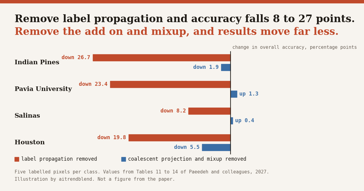
- Switching label propagation off costs 26.7, 23.4, 8.2 and 19.8 points. Switching off the coalescent projection and mixup together changes accuracy by down 1.85, up 1.26, up 0.41 and down 5.53 points, mostly inside one standard deviation.
- Label propagation runs over the unlabeled target pixels, which are also the test pixels. The authors say plainly that the method is transductive, and most listed baselines are not.
- The authors released code on GitHub. The PyTorch file in this article is our own small reconstruction on synthetic spectra, not their implementation.
Five pixels and a scene the model has never seen
Hyperspectral image classification assigns a land cover class to every pixel. Indian Pines separates corn, soybean and woods. Pavia University separates asphalt, meadows and bitumen inside a city. Salinas covers lettuce and vineyard plots, and Houston covers a university campus with roads, parking lots and a running track. Each scene comes from a different sensor, with a different number of bands and a different set of classes. A classifier trained on one rarely works on another.
Cross domain few shot learning, usually shortened to CDFSL, is the setting that tries to bridge that gap. The model first learns from a source scene that has plenty of labels. It then meets a target scene with a different set of classes and only a handful of labelled pixels for each. In this paper the source is Chikusei, a Japanese farmland and town scene with 19 classes and 77,592 labelled pixels. The four targets are Indian Pines with 16 classes, Pavia University with 9, Salinas with 16 and Houston with 15. The paper uses five labelled pixels per target class, and every other labelled pixel in the scene becomes the query set that the model must classify.
Training follows the episodic recipe common in few shot learning. Each episode draws a few classes, splits their samples into a support set with labels and a query set to be classified, builds one prototype per class from the support set, and scores each query pixel by its distance to those prototypes. The classifier is the prototypical network of Snell and colleagues, and it has no weights of its own, only an embedding network that decides which pixels land close together. The same episodic idea drives the prototype guided few shot medical segmentation method we analysed earlier.
| Scene | Role | Classes | Labelled pixels | Sensor and bands |
|---|---|---|---|---|
| Chikusei | Source | 19 | 77,592 | Headwall Hyperspec VNIR C, 128 bands |
| Indian Pines | Target | 16 | 10,249 | AVIRIS, 200 bands |
| Pavia University | Target | 9 | 42,776 | ROSIS, 103 bands |
| Salinas | Target | 16 | 54,129 | AVIRIS, 204 useful bands |
| Houston | Target | 15 | 15,029 (2,832 plus 12,197) | 144 bands, 2.5 metre pixels |
Class and pixel counts from Tables 1 to 5 of the paper. The Houston total is our sum of its training and testing columns. All scenes are reduced to 50 bands with principal component analysis and cut into 9 by 9 patches.
The authors name three weaknesses in earlier CDFSL work. Many methods enlarge the tiny target set with data augmentation such as added Gaussian noise, which they call unrealistic for hyperspectral data. Many train a lot of parameters from five examples per class, which invites overfitting. And very few use a foundation model pretrained on hyperspectral images. The only close precedent they cite uses DINOv2, a model trained on ordinary colour photos, with low rank adapters. MIFOMO is built to answer all three.
Three pieces on top of a frozen foundation model
The backbone stays untouched
The backbone is HyperSIGMA, a hyperspectral foundation model that was pretrained by masked image modelling on HyperGlobal 450K, a collection of 450 thousand hyperspectral images. It has two vision transformer branches. One treats spatial patches as tokens and the other treats groups of spectral bands as tokens. A spectral enhancement module fuses the two. The authors use the ViT B size and run only the first four layers of the spectral branch for fusion. Not one backbone weight changes during the few shot stages.
Freezing a large model is attractive when labels are scarce, because the pretrained features cannot be forgotten and there is little room to overfit. The price is that a frozen model needs some small adjustable part, or it cannot adapt to the target scene at all. Parameter efficient fine tuning methods supply that part. We covered the same idea for billion parameter vision models in Rein++, and the prompt based variant in BlackVIP. The paper adds a new one.
Coalescent projection, a matrix between query and key
Standard self attention builds queries and keys from the tokens, multiplies them, and turns the scores into weights. The coalescent projection, or CP, inserts one small learnable matrix between the query and the key in every attention head. With the same notation the paper uses, the head computes
Here \(C\) is a \(D’ \times D’\) matrix owned by that head. It starts close to the identity matrix, with ones on the diagonal and small random values of standard deviation 0.02 elsewhere, so the frozen model begins exactly where pretraining left it. Training then bends the similarity measure a little. A head that compared queries and keys with a plain dot product now compares them with a learned bilinear form.
The size works out cleanly. A ViT B head has dimension 64, so each matrix holds 4096 numbers. With 12 heads and 12 layers in each of the two branches, that gives 2 times 12 times 12 times 4096, which is 1,179,648, and it matches the figure in the paper’s parameter table. By the same arithmetic the paper’s LoRA count of 1,179,648 at rank 16 equals two branches, 12 layers and two adapted matrices, and its prompt count of 147,456 equals 8 prompt tokens, 768 dimensions and 24 layers. Those readings of the counts are ours, since the paper does not spell them out.
The authors frame CP as a generalization of the soft prompt. A prompt adds extra tokens that all heads share, so it needs a length chosen by hand and it enlarges the token sequence. CP gives every head its own matrix, needs no length, and keeps the sequence the same size. They also report that a single CP shared by all heads performs about as well, which we return to below.
| Way to adapt a frozen model | What is trained | Trainable parameters in the paper | Changes the token count |
|---|---|---|---|
| Coalescent projection | One matrix per head, between query and key | 1,179,648 | No |
| LoRA, rank 16 | Low rank updates to attention weights | 1,179,648 | No |
| Prompt, length 8 | Extra tokens shared across heads | 147,456 | Yes |
| Full fine tuning | The whole backbone | 171,683,073 in total | No |
From Table 28 of the paper. Every variant also trains 876,801 other parameters (the fusion module and small heads), except full fine tuning, where the 171,683,073 figure already includes them.
Mixup and an intermediate domain
Mixup creates a new training example by blending two real ones, and blending their labels in the same proportion. The paper uses it twice. In the source phase it mixes embeddings of source query pixels, which adds a second loss to the usual prototype loss. The mixing weight comes from a Beta distribution with both parameters set to 2.
The second use is the more novel one. The target scene has so few labels that the source and target are hard to align directly, so the method builds a bridge. It mixes source pixels with target pixels, at the input level and in embedding space, to form an intermediate domain. Because the two scenes have different classes, labels are padded into one joint label space, and a mixed example carries a weight on a source class and a weight on a target class.
The mixing ratio is not fixed. It starts near the target and drifts toward the source as training goes on, steered by a similarity term built from Wasserstein distances between the intermediate domain and each real domain, with a temperature of 0.05 and a random perturbation of 0.2. The intent is that the network masters the target first and the source second. No data augmentation is applied to the target scene, which is the paper’s answer to the first of its three complaints.
The target half of the bridge needs labels for target pixels, and there are none beyond the five per class. This is where the third piece enters.
Label propagation cleans the guesses
After training on the labelled target support pixels, the network guesses labels for the unlabeled target query pixels. Those pseudo labels are noisy. Label propagation, a classic graph method of Zhou and colleagues, smooths them. Every pixel becomes a node, edges carry a Gaussian similarity between embeddings, the graph is normalized, and labels flow along edges until they settle.
The paper sets \(\alpha\) to 0.9 and \(\sigma\) to 50. Each pixel’s final label is the class with the largest entry in its row of \(F^{*}\). The most confident predictions, the top 10 on Indian Pines and the top 100 elsewhere, are promoted into the support set that builds the intermediate domain. The authors also apply label propagation at every inference step, so the same smoothing shapes the final test predictions. That second use matters a great deal for how to read the results, and we come back to it.
In sequence, the recipe is three phases. Train on the source with prototype and mixup losses for 1500 episodes. Train on the five target support pixels per class, generate pseudo labels, clean them with label propagation and keep the confident ones. Then train on the intermediate domain for 500 to 1000 episodes while the mixing ratio slides. Training used one NVIDIA RTX 4090, and the MIFOMO numbers are averages over 20 random seeds.
What the numbers say
The headline results
On every one of the four target scenes, MIFOMO posts the highest overall accuracy in the paper’s comparison tables. The tables list between 10 and 17 competing methods per scene, from the classic SSRN network to recent cross domain few shot methods such as MGPDO, CFSL KT, CDLA and CASCL. The table below sets MIFOMO against the strongest listed baseline on each scene.
| Scene | Best listed baseline | Baseline OA | MIFOMO OA | Margin, our arithmetic | Margin in the paper’s text |
|---|---|---|---|---|---|
| Indian Pines | MGPDO | 81.32 ± 1.62 | 94.80 ± 4.44 | 13.5 points | 15 |
| Pavia University | MGPDO | 91.08 ± 1.07 | 97.35 ± 4.32 | 6.3 points | 7 |
| Salinas | CFSL KT | 95.13 ± 0.93 | 96.92 ± 5.21 | 1.8 points | 2 |
| Houston | CFSL KT | 82.63 ± 1.68 | 94.02 ± 3.3 | 11.4 points | 12 |
Overall accuracy in percent with five labelled pixels per class, from Tables 7 to 10 of the paper. MIFOMO figures are means over 20 seeds. The baseline figures are reported for 10 seeds, as taken from other papers. The abstract states margins of up to 14 percent.
The gaps are large on Indian Pines and Houston, moderate on Pavia University and small on Salinas. The authors ran t tests at the 0.05 level and report that MIFOMO is significantly better in every comparison except overall accuracy and kappa against CFSL KT on Salinas, which they call close. Their own rounding runs slightly generous. We make the margins 13.5, 6.3, 1.8 and 11.4 points where the text says 15, 7, 2 and 12, though the abstract’s up to 14 is consistent with the Indian Pines gap.
Where the gain comes from
Four ablation tables, one per target scene, switch the components on and off. The important rows are collected below. Every cell is overall accuracy with five labelled pixels per class.
| Configuration | Indian Pines | Pavia University | Salinas | Houston |
|---|---|---|---|---|
| Full MIFOMO | 94.80 | 97.35 | 96.92 | 94.02 |
| Without label propagation | 68.08 | 73.97 | 88.73 | 74.23 |
| Without coalescent projection | 94.56 | 96.74 | 96.26 | 93.92 |
| One CP shared by all heads | 94.56 | 98.42 | 97.50 | 94.31 |
| Without mixup | 94.51 | 99.22 | 96.99 | 93.81 |
| Without projection and without mixup | 92.95 | 98.61 | 97.33 | 88.49 |
From Tables 11 to 14 of the paper. Standard deviations for the full model are 4.44, 4.32, 5.21 and 3.3. Removing the coalescent projection means only the fusion module is trained in the few shot stages.
The pattern is stark. Dropping label propagation costs 26.7, 23.4, 8.2 and 19.8 points. Dropping the coalescent projection costs less than a point on every scene. Dropping mixup changes overall accuracy by down 0.29, up 1.87, up 0.07 and down 0.21 points. Removing both at once changes it by down 1.85, up 1.26, up 0.41 and down 5.53 points. Only the Houston scene shows a drop larger than the standard deviation of the full model. On Pavia University and Salinas, the variant with neither the projection nor mixup scores higher than the full method.
The full system is the best configuration on only one of the four scenes, and a single shared projection beats independent projections on three. These differences are small next to the 3 to 5 point seed to seed spread, so the fair reading is that the projection and mixup are about neutral on most scenes and clearly useful on Houston. The data do not support a claim that they drive the headline gains.
The authors read the same tables differently. They write that label propagation is central, which the numbers support, and that parameter efficient tuning through the projection contributes to gains on all datasets. The gains from the projection are 0.24, 0.61, 0.66 and 0.10 points, which supports that claim only weakly. The mixup claim is tied to Indian Pines and Houston, and the gains there are 0.29 and 0.21 points.
“Albeit promising performances of MIFOMO, it is as with other works in this domain categorized as the transductive approach, where a model has access to unlabeled samples of the target domain, i.e., the query set.”Paeedeh and colleagues, Conclusion
Label propagation by phase
Table 19 of the paper tracks accuracy after each training phase, with label propagation off and on. The paper presents it as pseudo label quality across the source, target and intermediate phases. The last column of each scene equals the headline number.
| Scene | After source phase | After target support phase | After intermediate phase | |||
|---|---|---|---|---|---|---|
| LP off | LP on | LP off | LP on | LP off | LP on | |
| Indian Pines | 60.87 | 92.55 | 66.73 | 93.92 | 68.08 | 94.80 |
| Pavia University | 72.77 | 98.28 | 72.68 | 97.17 | 73.97 | 97.35 |
| Salinas | 86.45 | 97.34 | 87.62 | 97.18 | 88.73 | 96.92 |
| Houston | 63.06 | 88.06 | 72.34 | 94.15 | 74.23 | 94.02 |
Overall accuracy in percent, from Table 19 of the paper. The highlighted cell marks the best value for each scene. LP stands for label propagation.
With label propagation on, a model that has only seen the source scene already reaches 92.55 on Indian Pines, 98.28 on Pavia University and 97.34 on Salinas. The later phases then add 2.25 points on Indian Pines and 5.96 on Houston, and they subtract 0.93 on Pavia University and 0.42 on Salinas. The paper says accuracy improves steadily across the three domains. By these numbers that holds on Indian Pines, and on Houston with a small step back after the middle phase. It does not hold on Pavia University or Salinas, where the best value comes earliest.
Without label propagation the intermediate phase does lift accuracy a little on all four scenes, by 7.2, 1.2, 2.3 and 11.2 points over the source phase. That is real evidence that mixup training helps the embedding. The effect is small beside the 8 to 32 point swing that label propagation delivers at every stage.
Is the projection a better way to tune
The paper compares the coalescent projection with LoRA, with prompt tuning and with full fine tuning of the backbone, keeping the rest of MIFOMO fixed.
| Tuning method | Indian Pines | Pavia University | Salinas | Houston |
|---|---|---|---|---|
| Coalescent projection | 94.80 | 97.35 | 96.92 | 94.02 |
| LoRA, rank 16 | 94.37 | 96.98 | 97.05 | 94.62 |
| Prompt, length 8 | 94.26 | 95.57 | 96.72 | 93.94 |
| Full fine tuning | 92.92 | 97.23 | 97.66 | 95.94 |
Overall accuracy in percent, from the lower rows of Tables 7 to 10. The paper bolds the full fine tuning result on Salinas and Houston.
The projection wins on Indian Pines and on Pavia University among the lightweight methods, and the gaps to LoRA are 0.43 and 0.37 points. On Salinas and Houston LoRA is ahead by 0.13 and 0.60 points, and full fine tuning is ahead by 0.74 and 1.92. The text states that the projection produces higher accuracies than LoRA across four datasets, which the table contradicts on two of them. The more defensible claim is that all three lightweight methods land within about two points of each other, and that the projection is a cheap one.
The cost side is where the projection looks good. Full fine tuning trains 171,683,073 parameters in total against 2,056,449 for the projection, a ratio of 83 by our arithmetic. The paper’s text says at least 8 times, which understates it. Training and memory figures follow.
| Tuning method | Train seconds, Indian Pines | Train seconds, Houston | Peak GPU memory, Indian Pines | Peak GPU memory, Houston |
|---|---|---|---|---|
| Coalescent projection | 483.25 | 392.73 | 3393 MB | 3343 MB |
| LoRA, rank 16 | 525.65 | 405.99 | 3410 MB | 3359 MB |
| Prompt, length 8 | 522.90 | 413.87 | 3546 MB | 3488 MB |
| Full fine tuning | 598.25 | 486.50 | 4807 MB | 4751 MB |
From Table 29 of the paper. Inference times are within about 0.7 seconds of each other on Indian Pines, 6.71 to 7.44 seconds.
Against full fine tuning the projection trains about 19 percent faster and uses about 29 percent less peak memory on both scenes shown. Those are useful savings, though not the 80 fold saving that the parameter count suggests. A likely reason, which is our inference and not the paper’s, is that the frozen backbone still runs forward and backward through every layer, so activations dominate the memory.
One more number deserves a mention. Inference time in Table 29 scales almost linearly with the number of query pixels. Dividing each inference time by its query set gives about 0.67, 0.65, 0.67 and 0.67 seconds per thousand pixels on Indian Pines, Pavia University, Salinas and Houston. This is our arithmetic, and it assumes the table covers the whole query set. It suggests that the label propagation solve, which Algorithm 1 runs on each mini batch of queries, does not blow up with scene size. It also means the result depends on the batch composition, and the batch size does not appear in the paper’s hyperparameter table.
Where the claims stretch
The comparison is not like for like
The authors defend the transductive setting by arguing that most baselines are transductive or use unrealistic data augmentation. The table’s characteristic column lets a reader check. Of the 17 methods in the Indian Pines table, our count finds that four involve transduction. Three more are tagged inductive and ten are tagged with augmentation only. CFSL KT, the closest baseline on Salinas and Houston, is transductive, and MGPDO, the best on the other two scenes, is tagged with augmentation.
“This should not affect the rigor of our experiments because most baseline approaches are also transductive approaches or make use of unrealistic data augmentations”Paeedeh and colleagues, Section 5.4
The ablation gives a way to test the argument. Without label propagation, our reading of the paper’s own tables puts MIFOMO at 68.08 on Indian Pines, which sits between SPRN at 67.32 and FDFSL at 71.11, and far under MGPDO at 81.32. On Pavia University the figure is 73.97, below every listed method, the lowest of which is SSRN at 76.78. On Salinas it is 88.73 against 89.13 for SSRN at the bottom of the list, and on Houston it is 74.23, above only SSRN at 68.23. The paper does not say outright that the cross mark also removes label propagation from inference, but the authors state that they apply it at every inference step, so we read the cross mark that way.
That reading says the frozen foundation model, the projection and the mixup training produce embeddings that are about as good as those of earlier methods, and that the large lead appears once a graph over the unlabeled test pixels is added. This is not an unfair thing to do, since transductive inference is a legitimate setting, and the authors state it plainly. It means that a practitioner who can only classify pixels one at a time should expect the lower row of the table and not the headline.
The Houston scene complicates this. CFSL KT is transductive too, and it trails MIFOMO by 11.4 points, and Houston is also the scene where removing the projection and mixup hurts most. So the pipeline is not just label propagation in a new coat, and the interaction between the embedding and the graph step clearly matters there. The honest summary is that label propagation does most of the lifting on most scenes and the rest of the pipeline matters most where the scene is hardest.
Variance and provenance
MIFOMO’s standard deviations run from 3.3 to 5.2 points on overall accuracy, while many baselines report 1 to 2 points. On Salinas the MIFOMO figure is 96.92 ± 5.21 against 95.13 ± 0.93 for CFSL KT. A method that is better on average but swings several times more from seed to seed is a different proposition for someone who gets one draw of five labelled pixels per class. The paper also states that MIFOMO used 20 seeds while the baselines carry 10 seeds as reported in other papers, so the baseline numbers were not rerun under one protocol. Preprocessing, splits and the choice of which pixels become labelled shots may differ between sources, and the paper does not claim otherwise.
Small classes
Indian Pines holds classes with 20, 28 and 46 labelled pixels in the whole scene. On those three, MIFOMO scores 85.65, 91.63 and 88.08 percent, while several baselines score 100. Its average accuracy of 90.75 is 4 points under its overall accuracy of 94.80, and the authors attribute low class accuracies to class imbalance in the scene. The gap between average and overall accuracy is a sign that the largest classes carry the headline.
The pretraining data
HyperSIGMA was pretrained on 450 thousand hyperspectral images, and the paper credits this breadth for the stable results. We could not find a statement about whether any of the four target scenes, or other imagery from the same flights or regions, appear in that pretraining set. Pretraining is self supervised and uses no labels, so this would not be label leakage, but it would bear on how unseen the target scenes really are. It is a question for the HyperSIGMA authors and for anyone reusing these benchmarks.
Two checks in the paper hold up well. Swapping the Chikusei source for the Kennedy Space Center scene moves accuracy on the four targets by less than 1 percentage point, which supports the idea that the backbone, not the source scene, carries the transfer. And the perturbation range, the temperature and the propagation spread all change accuracy by less than 1 point across the tested values. Only the trade off constant matters, and setting it to 0.5 gives notable drops.
Limitations the paper states, and the ones it leaves open
The paper states one limitation clearly. The method is transductive, so it needs access to the unlabeled query set of the target scene at inference time. The authors say their future work is the inductive setting, which they call much more challenging. We agree with the assessment and would add that the ablation numbers already give an early reading of how much harder it is.
The open questions are the ones this article has raised. How much of the lead survives under a single shared protocol with the same seeds and the same shot selection for every method. What the accuracy looks like when label propagation is given to the baselines too, since the technique is not specific to this model. How sensitive the results are to the mini batch size that shapes each graph. Whether the pretraining data overlap the target scenes. And how the method behaves on classes with a handful of pixels, where the baselines currently look better.
None of these is a reason to doubt the numbers in the tables, and the authors have released code at a public repository, which makes several of the checks easy for others to run. They are reasons to read the headline as a statement about a complete pipeline in a transductive setting, and not as a verdict on any one component.
A PyTorch version on synthetic spectra
The authors have published their implementation at a public repository, which is the right place to look for the real thing. What follows is our own independent reconstruction from the paper’s text and equations, written to show how the pieces fit together and to let a reader poke at them on a laptop. It is not their code, and it does not reproduce their numbers.
The file builds a small transformer over ten tokens of five spectral bands each, the same shape as 50 principal components. It pretrains that transformer by masked token reconstruction on unlabeled synthetic spectra, which stands in for HyperSIGMA, then freezes everything except one coalescent projection matrix per head. It then runs the three phases of the paper. The source phase uses the prototype loss plus embedding mixup. The target support phase trains on five labelled samples per class, split two and three. The intermediate phase mixes source and pseudo labelled target samples in input and embedding space with a sliding ratio. Label propagation uses the closed form of Eq. 21.
Several choices are ours, and the code marks each as a design choice. The data are synthetic class spectra with a band wise gain and offset shift between source and target, 12 source classes and 5 target classes. The graph bandwidth is local, set to half the mean distance to the ten nearest neighbours, because the paper’s value of 50 only makes sense on its own feature scale. We also normalize the propagated scores by class before taking the row maximum, a balancing step the paper does not describe. The backbone is a toy with 32 dimensions, 4 heads and 2 layers.
"""
MIFOMO style cross domain few shot learning, a small reference reconstruction.

Written by aitrendblend from the published description in Paeedeh et al.,
Neural Networks 206 (2027) 109684. It is NOT the authors' code. Their
implementation is public at https://github.com/Naeem-Paeedeh/MIFOMO.

What this file shows
  1. Coalescent projection (CP): one learnable matrix per attention head,
     placed between the query and key, on top of a frozen transformer.
  2. Prototype loss with embedding space mixup (source phase).
  3. Label propagation with the closed form F = (I - alpha S)^-1 Y.
  4. Intermediate domain training with the adaptive mixup ratio.
  5. A smoke test on synthetic spectral data with a domain shift.

Stand ins (the paper uses real data and a real foundation model)
  * The backbone is a tiny transformer over band group tokens, pretrained with
    masked token reconstruction on unlabeled synthetic data. It stands in for
    HyperSIGMA. It is frozen before any few shot training.
  * Data are synthetic class spectra with a band wise gain and offset shift.
Design choices the paper does not fix are marked DESIGN.
"""
import math
import torch
import torch.nn as nn
import torch.nn.functional as F

torch.manual_seed(0)
DEV = "cpu"

# ----------------------------------------------------------------------------
# Synthetic spectral data
# ----------------------------------------------------------------------------
BANDS, GROUP = 50, 5                  # 10 tokens of 5 bands, like PCA 50 bands
N_TOK = BANDS // GROUP


def make_domain(n_classes, per_class, shift, gen, noise=0.55):
    """Smooth class spectra plus noise. `shift` applies a band wise gain/offset."""
    t = torch.linspace(0, 1, BANDS)
    protos = []
    for _ in range(n_classes):
        f = torch.rand(3, generator=gen) * 6 + 1
        p = torch.rand(3, generator=gen) * 6.28
        a = torch.rand(3, generator=gen) + 0.3
        protos.append(sum(a[i] * torch.sin(f[i] * t * 3.14 + p[i]) for i in range(3)))
    protos = torch.stack(protos)
    gain = 1 + shift * (torch.rand(BANDS, generator=gen) - 0.5) * 2
    off = shift * (torch.rand(BANDS, generator=gen) - 0.5) * 1.0
    x, y = [], []
    for c in range(n_classes):
        base = protos[c] * gain + off
        x.append(base + noise * torch.randn(per_class, BANDS, generator=gen))
        y.append(torch.full((per_class,), c))
    return torch.cat(x), torch.cat(y)


# ----------------------------------------------------------------------------
# Transformer with optional coalescent projection
# ----------------------------------------------------------------------------
class Attn(nn.Module):
    def __init__(self, d, heads, use_cp=False, cp_sigma=0.02):
        super().__init__()
        self.h, self.dh = heads, d // heads
        self.qkv = nn.Linear(d, 3 * d)
        self.out = nn.Linear(d, d)
        self.use_cp = use_cp
        if use_cp:
            # Eq 13: identity plus N(0, sigma) noise, one matrix per head
            c = torch.eye(self.dh).repeat(heads, 1, 1)
            c = c + cp_sigma * torch.randn_like(c) * (1 - torch.eye(self.dh))
            self.cp = nn.Parameter(c)

    def forward(self, x):
        b, n, d = x.shape
        q, k, v = self.qkv(x).view(b, n, 3, self.h, self.dh).permute(2, 0, 3, 1, 4)
        if self.use_cp:
            q = q @ self.cp                       # Q C, per head (Eq 11)
        att = torch.softmax(q @ k.transpose(-1, -2) / math.sqrt(self.dh), -1)
        return self.out((att @ v).transpose(1, 2).reshape(b, n, d))


class Block(nn.Module):
    def __init__(self, d, heads, use_cp):
        super().__init__()
        self.n1, self.n2 = nn.LayerNorm(d), nn.LayerNorm(d)
        self.attn = Attn(d, heads, use_cp)
        self.mlp = nn.Sequential(nn.Linear(d, 4 * d), nn.GELU(), nn.Linear(4 * d, d))

    def forward(self, x):
        x = x + self.attn(self.n1(x))
        return x + self.mlp(self.n2(x))


class Backbone(nn.Module):
    def __init__(self, d=32, heads=4, depth=2, use_cp=True):
        super().__init__()
        self.embed = nn.Linear(GROUP, d)
        self.pos = nn.Parameter(torch.randn(1, N_TOK, d) * 0.02)
        self.blocks = nn.ModuleList([Block(d, heads, use_cp) for _ in range(depth)])
        self.norm = nn.LayerNorm(d)
        self.recon = nn.Linear(d, GROUP)          # only for masked pretraining

    def tokens(self, x):
        return self.embed(x.view(-1, N_TOK, GROUP)) + self.pos

    def forward(self, x, tok=None):
        z = self.tokens(x) if tok is None else tok
        for blk in self.blocks:
            z = blk(z)
        return self.norm(z).mean(1)               # pooled embedding


def pretrain_mae(bb, data, steps=300, mask=0.5):
    """Masked token reconstruction. Stand in for HyperSIGMA pretraining."""
    opt = torch.optim.Adam(bb.parameters(), 2e-3)
    for _ in range(steps):
        x = data[torch.randint(len(data), (128,))]
        tok = bb.tokens(x)
        m = (torch.rand(x.shape[0], N_TOK) < mask).unsqueeze(-1)
        z = torch.where(m, torch.zeros_like(tok), tok)
        for blk in bb.blocks:
            z = blk(z)
        rec = bb.recon(bb.norm(z))
        tgt = x.view(-1, N_TOK, GROUP)
        loss = ((rec - tgt) ** 2 * m).sum() / (m.sum() * GROUP + 1e-8)
        opt.zero_grad(); loss.backward(); opt.step()
    return float(loss.detach())


def freeze_except_cp(bb):
    for n, p in bb.named_parameters():
        p.requires_grad = n.endswith(".cp")
    return sum(p.numel() for p in bb.parameters() if p.requires_grad)


# ----------------------------------------------------------------------------
# Prototype loss with embedding space mixup
# ----------------------------------------------------------------------------
def prototypes(emb, y, n_cls):
    return torch.stack([emb[y == c].mean(0) for c in range(n_cls)])


def proto_logits(emb, protos):
    return -torch.cdist(emb, protos) ** 2          # Eq 3, squared Euclidean


def soft_ce(logits, soft):
    return -(soft * F.log_softmax(logits, -1)).sum(-1).mean()


def mixup_embed_loss(emb, y_soft, protos, alpha=2.0):
    """Eq 14 to 15, mix pairs of embeddings and their soft labels."""
    lam = torch.distributions.Beta(alpha, alpha).sample((emb.shape[0], 1))
    perm = torch.randperm(emb.shape[0])
    e = lam * emb + (1 - lam) * emb[perm]
    ys = lam * y_soft + (1 - lam) * y_soft[perm]
    return soft_ce(proto_logits(e, protos), ys)


def sample_episode(x, y, n_cls, k_sup, k_qry, gen=None):
    sx, sy, qx, qy = [], [], [], []
    for c in range(n_cls):
        idx = (y == c).nonzero().squeeze(1)
        idx = idx[torch.randperm(len(idx))]
        sx.append(x[idx[:k_sup]]); sy += [c] * k_sup
        qx.append(x[idx[k_sup:k_sup + k_qry]]); qy += [c] * k_qry
    return torch.cat(sx), torch.tensor(sy), torch.cat(qx), torch.tensor(qy)


# ----------------------------------------------------------------------------
# Label propagation, Eq 20 and 21
# ----------------------------------------------------------------------------
def label_propagation(emb_sup, y_sup, emb_qry, n_cls, alpha=0.9, sigma=None):
    """Closed form F = (I - alpha S)^-1 Y over support + query nodes.
    Returns normalized scores for the query rows."""
    z = torch.cat([emb_sup, emb_qry])
    d2 = torch.cdist(z, z) ** 2
    if sigma is None:                              # DESIGN: local bandwidth
        sigma = 0.5 * d2.sort(1).values[:, 1:11].mean().sqrt()
    a = torch.exp(-d2 / (2 * sigma ** 2))
    a.fill_diagonal_(0)                            # a_ii = 0
    dinv = a.sum(1).clamp_min(1e-8).pow(-0.5)
    s = dinv[:, None] * a * dinv[None, :]          # D^-1/2 A D^-1/2
    y = torch.zeros(z.shape[0], n_cls)
    y[torch.arange(len(y_sup)), y_sup] = 1.0       # support rows one hot
    f = torch.linalg.solve(torch.eye(z.shape[0]) - alpha * s, y)
    f = f[len(y_sup):]
    f = f / f.sum(0, keepdim=True).clamp_min(1e-12)   # DESIGN: class balance
    return f / f.sum(1, keepdim=True).clamp_min(1e-12)


# ----------------------------------------------------------------------------
# Three phase training
# ----------------------------------------------------------------------------
def embed(bb, x):
    return bb(x)


def source_phase(bb, xs, ys, n_src, episodes=150, lr=3e-3):
    opt = torch.optim.Adam([p for p in bb.parameters() if p.requires_grad], lr)
    for _ in range(episodes):
        sx, sy, qx, qy = sample_episode(xs, ys, n_src, 5, 10)
        ps = prototypes(embed(bb, sx), sy, n_src)
        eq = embed(bb, qx)
        l_fsl = F.cross_entropy(proto_logits(eq, ps), qy)               # Eq 15
        l_mx = mixup_embed_loss(eq, F.one_hot(qy, n_src).float(), ps)
        loss = l_fsl + l_mx                                             # Eq 16
        opt.zero_grad(); loss.backward(); opt.step()


def target_support_phase(bb, xt, yt_sup_idx, n_tgt, episodes=60, lr=3e-3):
    """Train on the 5 labelled target samples per class only (2/5 and 3/5 split)."""
    opt = torch.optim.Adam([p for p in bb.parameters() if p.requires_grad], lr)
    sx, sy = xt[yt_sup_idx[0]], yt_sup_idx[1]
    for _ in range(episodes):
        perm = torch.randperm(len(sy))
        a, b = [], []
        for c in range(n_tgt):
            idx = (sy[perm] == c).nonzero().squeeze(1)
            a.append(perm[idx[:2]]); b.append(perm[idx[2:]])
        a, b = torch.cat(a), torch.cat(b)
        ps = prototypes(embed(bb, sx[a]), sy[a], n_tgt)
        eq = embed(bb, sx[b])
        loss = F.cross_entropy(proto_logits(eq, ps), sy[b]) + \
            mixup_embed_loss(eq, F.one_hot(sy[b], n_tgt).float(), ps)
        opt.zero_grad(); loss.backward(); opt.step()


@torch.no_grad()
def pseudo_label(bb, sx, sy, qx, n_tgt, topk, use_lp=True):
    es, eq = embed(bb, sx), embed(bb, qx)
    if use_lp:
        scores = label_propagation(es, sy, eq, n_tgt)
    else:
        scores = torch.softmax(proto_logits(eq, prototypes(es, sy, n_tgt)), -1)
    conf, lab = scores.max(1)
    keep = conf.argsort(descending=True)[:topk]
    return lab, keep


def lam_update(lam_prev, epoch, n_epochs, q):                 # Eq 25
    return epoch * (1 - q) / n_epochs + q * lam_prev


def intermediate_phase(bb, xs, ys, n_src, sx_t, sy_t, qx_t, plab, keep, n_tgt,
                       episodes=80, lr=3e-3, tau=0.05, sigma=0.2, lam0=0.1):
    """Mix source and (pseudo labelled) target in input and embedding space.
    Joint label space of size n_src + n_tgt realizes the padding strategy."""
    opt = torch.optim.Adam([p for p in bb.parameters() if p.requires_grad], lr)
    k = n_src + n_tgt
    tx = torch.cat([sx_t, qx_t[keep]])
    ty = torch.cat([sy_t, plab[keep]]) + n_src
    lam, n_ep = lam0, 4
    per = episodes // n_ep
    for ep in range(1, n_ep + 1):
        for _ in range(per):
            sx, sy, _, _ = sample_episode(xs, ys, n_src, 5, 0)
            allx = torch.cat([sx, tx]); ally = torch.cat([sy, ty])
            protos = prototypes(embed(bb, allx), ally, k)
            lam_t = (lam + (torch.rand(1) * 2 - 1) * sigma).clamp(0, 1)   # Eq 26
            i = torch.randint(len(sx), (64,)); j = torch.randint(len(tx), (64,))
            ys_oh = F.one_hot(sy[i], k).float(); yt_oh = F.one_hot(ty[j], k).float()
            x_mix = lam_t * sx[i] + (1 - lam_t) * tx[j]                    # Eq 22
            e_in = embed(bb, x_mix)
            e_em = lam_t * embed(bb, sx[i]) + (1 - lam_t) * embed(bb, tx[j])  # Eq 23
            y_mix = lam_t * ys_oh + (1 - lam_t) * yt_oh
            loss = soft_ce(proto_logits(e_in, protos), y_mix) + \
                soft_ce(proto_logits(e_em, protos), y_mix)                # Eq 27
            opt.zero_grad(); loss.backward(); opt.step()
        with torch.no_grad():                                              # Eq 24
            d_s = (embed(bb, xs[:200]).mean(0) - embed(bb, x_mix).mean(0)).norm()
            d_t = (embed(bb, tx).mean(0) - embed(bb, x_mix).mean(0)).norm()
            q = torch.exp(-d_s / (d_s + d_t + 1e-8) / tau).item()
        lam = lam_update(lam, ep, n_ep, q)


@torch.no_grad()
def evaluate(bb, sx, sy, qx, qy, n_tgt, use_lp):
    es, eq = embed(bb, sx), embed(bb, qx)
    if use_lp:
        pred = label_propagation(es, sy, eq, n_tgt).argmax(1)
    else:
        pred = proto_logits(eq, prototypes(es, sy, n_tgt)).argmax(1)
    return (pred == qy).float().mean().item() * 100


# ----------------------------------------------------------------------------
# Parameter accounting
# ----------------------------------------------------------------------------
def count_params(d=32, heads=4, depth=2, rank=4):
    dh = d // heads
    return {
        "coalescent projection": depth * heads * dh * dh,
        "shared prompt (len 8)": 8 * d,
        "LoRA on q, k, v and out": depth * 4 * rank * 2 * d,
        "full attention weights": depth * (3 * d * d + 3 * d + d * d + d),
    }


# ----------------------------------------------------------------------------
# Smoke test
# ----------------------------------------------------------------------------
def run(seed):
    g = torch.Generator().manual_seed(seed)
    torch.manual_seed(seed)
    xs, ys = make_domain(12, 200, shift=0.0, gen=g)
    xt, yt = make_domain(5, 150, shift=0.8, gen=g)
    bb = Backbone(use_cp=True)
    pretrain_mae(bb, torch.cat([xs, xt]))        # unlabeled pool, stands in for HyperSIGMA
    n_cp = freeze_except_cp(bb)
    source_phase(bb, xs, ys, 12)
    # five labelled target samples per class
    sup_idx, qry_idx = [], []
    for c in range(5):
        idx = (yt == c).nonzero().squeeze(1)
        idx = idx[torch.randperm(len(idx))]
        sup_idx.append(idx[:5]); qry_idx.append(idx[5:])
    sup_idx, qry_idx = torch.cat(sup_idx), torch.cat(qry_idx)
    sx, sy, qx, qy = xt[sup_idx], yt[sup_idx], xt[qry_idx], yt[qry_idx]
    out = {"cp_params": n_cp}
    out["source_only_oa"] = evaluate(bb, sx, sy, qx, qy, 5, False)
    out["source_only_lp_oa"] = evaluate(bb, sx, sy, qx, qy, 5, True)
    target_support_phase(bb, xt, (sup_idx, sy), 5)
    for use_lp in (False, True):
        lab, keep = pseudo_label(bb, sx, sy, qx, 5, topk=100, use_lp=use_lp)
        out[f"pseudo_acc_lp{int(use_lp)}"] = (lab[keep] == qy[keep]).float().mean().item() * 100
    lab, keep = pseudo_label(bb, sx, sy, qx, 5, topk=100, use_lp=True)
    intermediate_phase(bb, xs, ys, 12, sx, sy, qx, lab, keep, 5)
    out["final_no_lp_oa"] = evaluate(bb, sx, sy, qx, qy, 5, False)
    out["final_lp_oa"] = evaluate(bb, sx, sy, qx, qy, 5, True)
    return out


if __name__ == "__main__":
    print("Parameter counts for a d=32, 4 head, 2 layer toy backbone")
    for k, v in count_params().items():
        print(f"  {k:28s} {v:7d}")
    rows = [run(s) for s in range(3)]
    keys = [k for k in rows[0] if k != "cp_params"]
    print(f"\nTrainable CP parameters: {rows[0]['cp_params']}")
    print("Mean over 3 seeds, target accuracy in percent")
    for k in keys:
        vals = torch.tensor([r[k] for r in rows])
        print(f"  {k:22s} {vals.mean():6.2f} +/- {vals.std():5.2f}")
    # basic sanity checks
    assert rows[0]["cp_params"] == 2 * 4 * 8 * 8
    mean = lambda k: sum(r[k] for r in rows) / len(rows)
    assert mean("final_lp_oa") > mean("final_no_lp_oa") - 1.0
    assert mean("pseudo_acc_lp1") > 80.0
    print("\nsmoke test passed")
The smoke test prints parameter counts, then runs three seeds of the whole pipeline and prints mean target accuracy at each stage, with and without label propagation.
The parameter counts mirror the paper’s pattern at toy scale. The projection trains 512 numbers, 6 percent of the 8448 attention weights, a shared prompt of length 8 would train 256, and rank 4 LoRA on all four attention matrices would train 2048. The ordering differs from the paper’s table, where the projection matches LoRA, because our rank 4 choice is arbitrary. The point is the scale, a few hundred numbers against thousands.
The accuracy lines tell a story close to the paper’s. A model trained only on the source scene classifies the five target classes at 88.05 percent. Switching label propagation on lifts it to 95.54. The target and intermediate phases then add 4.5 points without propagation and 1.7 with it, ending at 92.51 and 97.20. The two helpers stack, but the graph step is the larger single effect at the first stage, and the later training matters most when propagation is off. Pseudo label accuracy for the 100 most confident samples is 100 percent either way, so our toy is too easy to show propagation cleaning noisy guesses, and the benefit shows only at evaluation.
The toy also taught us something the paper plays down. In a quick sweep that we ran while building it, the bandwidth of the graph moved target accuracy anywhere from 44.7 to 98.1 percent across 12 settings and three seeds. The first version of our code used the median pairwise distance as the bandwidth, and label propagation made things worse, with accuracy dropping from 88 to 55 percent. The paper reports that its spread parameter has a negligible effect. That is plausible if its embeddings are normalized to a scale where 50 is sensible, and it is a reminder that the graph step is where careful tuning hides. Anyone reimplementing the method should check the feature scale first.
Label propagation turns a handful of labels into a smooth assignment over every unlabeled pixel, and it is very sensitive to how the graph is built. If you reuse the method, treat the bandwidth, the batch that forms each graph and the class balancing as part of the model, and report them.
What this adds up to
The paper’s contribution is a clear recipe for few label hyperspectral classification. Take a foundation model that has seen hundreds of thousands of images, freeze it, tune a small matrix inside each attention head, bridge the source and target scenes with mixup, and clean the target guesses with a graph. On four standard benchmarks and with five labelled pixels per class, the full pipeline posts overall accuracy between 94.02 and 97.35 percent and leads the listed baselines on every scene. The authors release their code, run a t test, test an alternative source scene and sweep their hyperparameters, which is more transparency than many papers in this area offer.
The ablation tables carry the sharper message. Switching label propagation off drops accuracy by 8.2 to 26.7 points, while removing the coalescent projection and mixup together changes it by between up 1.26 and down 5.53 points, mostly inside the seed to seed spread. The foundation model, the projection and mixup produce an embedding that is competitive with earlier methods when classifying one pixel at a time, and the large lead appears when a graph over the unlabeled test pixels is added. That is a useful finding, and it differs from the story the title and abstract tell.
The coalescent projection itself deserves a fair hearing. It is a neat idea, one matrix per head with an identity start, that adds no tokens and no hyperparameter beyond its noise scale. It trains 19 percent faster and with 29 percent less memory than full fine tuning of the backbone, and it beats full fine tuning on Indian Pines, matches it on Pavia University and trails it by 0.74 and 1.92 points on Salinas and Houston. What the evidence does not show is that it beats LoRA, which is ahead on Salinas and Houston, or that it drives the headline gain. A larger and cleaner comparison would settle that, and the open repository makes such a comparison easy.
The conditions of the comparison deserve the same care. MIFOMO’s averages come from 20 seeds, while the baselines carry 10 seeds taken from other papers, and its seed to seed spread is two to six times larger than that of the strongest baselines. Most of the strongest baselines are not tagged as transductive, while MIFOMO’s best numbers rely on a transductive step that the authors apply at every inference. The authors say so plainly, and the point is not misconduct but context. A user who must label pixels one at a time, or who cannot see the full target scene in advance, should expect the lower rows of the ablation table.
The wider lesson is about where the effort in few shot learning goes. Readers who follow remote sensing will find related threads in our coverage of SSA Mamba for hyperspectral classification and of an information bottleneck for hyperspectral and LiDAR fusion, and more analyses on attention models sit in the vision transformers and attention archive. Foundation models promise that pretrained features generalize, and the paper is partly a test of that promise. The evidence here is encouraging, since swapping the source scene changes accuracy by under a point, yet the biggest single gain comes from a classic graph method from 2003 that exploits the structure of the unlabeled data. Large pretrained models and old fashioned smoothing are not rivals, and the best results seem to need both. Papers that report both, and report what happens without each, are the ones that teach the most.
The authors name the inductive setting as their next step, and we would watch it closely. A method that keeps most of its accuracy without ever seeing the unlabeled test pixels would settle most of the doubts raised here. Until then, the safest reading is that MIFOMO is a strong transductive pipeline for hyperspectral scenes with five labelled pixels per class, whose reported gains are driven mainly by label propagation, and whose lighter components are cheap, tidy and about neutral on most of the scenes tested.
Frequently asked questions
What is MIFOMO and what problem does it solve?
MIFOMO classifies hyperspectral image pixels in a new scene when only five labelled pixels per class are available. It freezes the HyperSIGMA foundation model, tunes a small matrix inside each attention head called the coalescent projection, bridges a source scene and the target scene with mixup, and cleans noisy pseudo labels with label propagation.
How accurate is it with five labelled pixels per class?
The paper reports overall accuracy of 94.80 percent on Indian Pines, 97.35 on Pavia University, 96.92 on Salinas and 94.02 on Houston. By our arithmetic these beat the strongest listed baseline by 13.5, 6.3, 1.8 and 11.4 points. MIFOMO’s seed to seed standard deviations of 3.3 to 5.2 points are larger than those of many baselines.
What does the coalescent projection do?
It is one learnable matrix per attention head, inserted between the query and the key and started near the identity. In the paper’s ViT B setting it adds 1,179,648 trainable parameters while the backbone stays frozen. It trains about 19 percent faster than full fine tuning, and removing it changes accuracy by less than a point on every scene in the paper’s ablations.
How much does label propagation matter?
Removing it lowers overall accuracy by 26.7, 23.4, 8.2 and 19.8 points on the four scenes. Removing the coalescent projection and mixup together changes accuracy by down 1.85, up 1.26, up 0.41 and down 5.53 points. Label propagation is also applied at inference over the unlabeled test pixels, which makes the method transductive.
Is the comparison with other methods fair?
Only partly. The authors say MIFOMO is transductive and argue that most baselines are too or use augmentation, but our count of the Indian Pines table finds four of 17 methods involve transduction. The baseline numbers come from other papers with 10 seeds while MIFOMO uses 20. Without label propagation MIFOMO scores 68.08 on Indian Pines against 81.32 for the best baseline.
Can I run the code?
Yes. The authors released their implementation at a public GitHub repository, linked below. The PyTorch file on this page is a separate reconstruction on synthetic spectra that runs in under a minute on a CPU. It shows the mechanics of the coalescent projection, mixup and label propagation, and it does not reproduce the paper’s numbers.
Read the paper and run the authors’ code
The article is open access under a Creative Commons license in Neural Networks. The authors host their implementation on GitHub, so the second button leads to the original code and not to our toy reconstruction.
Paeedeh, N., Pratama, M., Shiddiqi, A., Cao, Z., Prasad, M., and Jatmiko, W. Cross domain few shot learning for hyperspectral image classification based on mixup foundation model. Neural Networks 206 (2027) 109684. DOI 10.1016/j.neunet.2026.109684. Open access under a CC BY license.
This analysis is based on the published paper and an independent evaluation of its claims.