
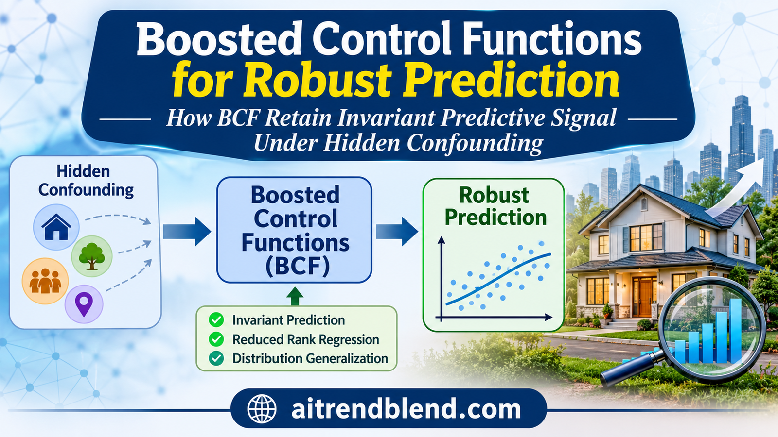
A model trained on one part of California predicts house values well nearby, then struggles when asked to predict another region. The recorded features still look familiar. What changed is how those features relate to unmeasured influences on the outcome. The paper behind boosted control functions asks which parts of that predictive relationship can survive a specified change in environment, even when the underlying causal function cannot be recovered uniquely.
- The boosted control function targets robust prediction under a defined family of shifts rather than identifying every causal effect.
- It combines a structural component with stable predictive information recovered from a control function.
- The invariant coordinates come from the left null space of the map linking exogenous variables to predictors.
- Its population guarantee requires identification, support or extrapolation conditions, and a sufficiently rich shift family.
- ControlTwicing estimates additive components through repeated regressions, followed by a separate invariant correction.
- The housing experiment supports a qualified robustness comparison, with different methods winning different geographic splits.
This article explains published research and is not medical advice, diagnosis or treatment. Consult a qualified professional about health decisions. The paper mentions hospitals as a possible environment label, but its reported real data experiment concerns housing. It provides no patient cohort, diagnostic performance or clinical validation, and no clinical review has been supplied.
Predicting through a shift is not the same as recovering causation
Nicola Gnecco at Imperial College London, Jonas Peters at ETH Zurich, Sebastian Engelke at the University of Geneva and Niklas Pfister at the University of Copenhagen develop the framework in Boosted Control Functions, published in JMLR. The work connects distribution generalization with simultaneous equation models and control function ideas from econometrics.
The starting problem is prediction with hidden confounding. Unobserved variables can influence both a recorded predictor and the response. A flexible regression model can exploit that association successfully in its training distribution. If the process generating the recorded predictors changes, the same association may become less useful or misleading.
A common response is to seek the structural function that describes how the response depends on the predictors. The paper shows why prediction can have a different target. Some confounding related information remains stable under the allowed shifts. A predictor may use that stable information without claiming that it represents a causal effect of changing a predictor.
This is a Machine Learning analysis of what a prediction target should be under uncertainty about the deployment distribution. The distinction matters alongside our discussion of experimental design for causal identification. Good prediction under a model of changing environments and identification of an intervention effect answer separate questions.
Specify what changes before claiming robustness
The framework uses a structural response equation and a reduced form equation for the predictors. An observed exogenous vector changes the predictors through a linear map. The unobserved terms in the two equations may be dependent, which permits confounding. Their joint distribution is independent of the exogenous variables and stays fixed across the environments considered.
Here the columns of \(M_0\) identify the directions in predictor space that the exogenous variables can move. Training and testing differ through the distribution of \(Z\). The response function, this linear map and the joint noise law remain fixed. Confounding means that knowing the predictor noise can reveal information about the response noise.
This is more specific than an arbitrary distribution shift. It excludes an unexplained change in the response mechanism or in the joint confounding law. The paper discusses extensions through known feature maps of the exogenous variables, but it does not offer unrestricted generalization for an unknown nonlinear first stage. Declaring a variable exogenous is also a substantive assumption, not an output of ordinary regression.
At training time the observations include predictors, outcomes and exogenous variables. At prediction time the method is designed to use the predictors alone. An environment label can become unavailable because a new category appears. A continuous geographic variable may remain recorded yet be difficult to use directly when extrapolating into a region outside the training geography.
The framework can accommodate certain direct linear effects of the exogenous variables after a suitable reexpression of the equations. This requires the paper’s projectability condition. It should not be read as permission for arbitrary direct effects of environment on outcome. A site label that represents several unmodeled mechanisms does not become valid merely because it has been encoded as a number.
Training residual independence can miss the relevant failure
The paper defines strong invariance through the full distribution of the prediction residual. An invariant function produces the same residual law under every distribution in the specified family. This is stronger than asking whether a residual has zero correlation with an environment variable on the training sample.
The distinction is especially revealing for nonlinear functions. The paper constructs an example in which training environments take the values \(-2\pi\) and \(2\pi\). Adding a sine term to the structural function does not reveal dependence on those training labels because the periodic shifts cancel. Moving the exogenous variable to \(\pi\) reverses the sine term and changes the residual distribution.
Residual independence in the observed environments can therefore coexist with failure in an allowed new environment. The paper also gives conditions under which the weaker and stronger notions coincide, so the message is not that independence is always useless. The point is to match an invariance diagnostic with the support and function assumptions that make it informative.
This also explains why an attractive residual plot cannot prove the population guarantee. A finite set of observed environments does not enumerate every possible shift in the model family. Empirical residual checks can identify failures, but passing them is not a general certificate that the right function has been recovered.
The null space locates the stable information
Let the first stage map have rank \(q\), with \(p\) recorded predictors. If the rank is smaller than the number of predictors, some linear combinations of those predictors cannot be changed by moving the exogenous variables. An orthonormal basis for the left null space identifies these combinations.
The last equality supplies the mechanism. Projecting the predictors into these coordinates removes the term driven by \(Z\). Those coordinates depend only on the predictor noise, whose distribution remains fixed across the allowed environments. They can carry information about the response noise when hidden confounding is present.
The stable coordinates do not make the other predictor directions irrelevant. The structural part of the response may depend on every coordinate. The final predictor therefore retains a structural component and adds a correction based on the invariant coordinates. Simply discarding all directions affected by the exogenous variables would be a different method.
When the first stage has full row rank, there is no nontrivial invariant coordinate space. In that limiting case, the population correction reduces to the mean of the control function, which is zero under the model assumptions. The boosted control function then coincides with the structural function.
Why an unidentified decomposition can still yield an identified predictor
The control function is the conditional mean of the response noise given the predictor noise. Once the control variable is available, the conditional response mean separates into a function of the predictors and a function of that control variable.
With insufficient rank, that decomposition need not be unique. A function of the invariant coordinates can be moved from one component to the other without changing their sum on the observed distribution. Estimating the additive conditional mean well therefore does not necessarily identify the causal response function.
The boosted control function compensates for this ambiguity. It adds the part of the control function that can be predicted from the invariant coordinates. Under the identification conditions, changing the additive decomposition changes the two contributions in opposite directions, leaving the final prediction unchanged.
This is the central contribution. The stable prediction target can be identified even when the structural component alone is not. Confounding is not treated as information that must all be thrown away. Its use is restricted to the part compatible with the stated shift family.
The identification conditions are substantial. For categorical exogenous variables, one sufficient route uses a linear control function, nonzero category probabilities and overlap and spanning conditions. A second route allows differentiable structural and control functions with conditions on the support of the continuous variables. Neither route says that arbitrary labels and unrestricted neural networks automatically identify the target.
Separate the target from its decomposition. The estimated structural component may vary between valid fits. What matters for BCF is whether the final structural component plus invariant correction is identified under the stated assumptions.
The robustness guarantee has a measurable price
The ideal least squares predictor uses every training distribution association available in the predictors. If there is no distribution change, it is optimal for squared error. The boosted control function restricts how it uses the confounding related part of that information. Proposition 13 makes the resulting training risk cost explicit.
The extra term is nonnegative. Robustness does not arrive as a universal improvement on the original distribution. It can require giving up a useful but unstable shortcut. That tradeoff is more informative than a claim that a robust method should win on every test set, including a test set drawn from training conditions.
“the price one needs to pay in terms of prediction performance to be invariant”Gnecco, Peters, Engelke and Pfister, discussion following Proposition 13.
Theorem 15 gives a minimax statement when the function and shift assumptions hold. The BCF minimizes the worst risk over the specified distribution family. A richness condition ensures that the family includes environments strong enough to remove the usefulness of unstable confounding information. The paper provides sufficient examples involving increasingly variable Gaussian shifts.
Support also matters. The analysis requires either a suitable domination condition or a function class condition ensuring that functions agreeing in training continue to agree in the target family. Generalization outside observed support does not appear without restrictions. The theorem also relies on the stated moment conditions and fixed mechanisms.
The guarantee is about the population target. An estimated neural network can miss it because the first stage is noisy, the additive regressions are inaccurate or the final correction is poorly fitted. Our article on robust regression error estimation concerns another statistical problem, but the same reading discipline applies. A characterized estimand and a fitted finite sample model are separate objects.
ControlTwicing estimates the components before adding the correction
The practical procedure first estimates the predictor response to the exogenous variables through reduced rank regression. It penalizes the rank of the first stage map and chooses a penalty through cross validation. The estimated control variable is the residual after removing this fitted exogenous contribution. An SVD then yields the estimated invariant basis.
ControlTwicing alternates two regressions. It initially regresses the centered response on the estimated controls. It then regresses the response minus the fitted control function on the predictors. Subsequent passes alternate those two fits using the current residual. Each pass replaces a component fit rather than adding every previous fitted function to the final predictor.
The correction is a separate regression after this alternation. The fitted control function values are regressed on the estimated invariant coordinates. At prediction time the method adds that fitted correction to the learned predictor component. It does not require a test observation’s exogenous vector to reconstruct its control residual.
Appendix E provides a neural alternative. Two networks jointly fit the additive conditional mean, followed by a correction network trained on the remaining response residual using the invariant coordinates. The appendix’s prose identifies those coordinates as the correction input, even though a displayed loss has an inconsistent argument. The reference code follows the stated conditional expectation, with no correction that depends directly on an unavailable test control variable.
The convergence discussion in Appendix B uses sample splitting and treats the first stage quantities as known. It bounds the overall rate through the slower of the two regression stages considered there. The paper identifies extension to estimated first stage quantities as future work. That limitation matters when presenting a complete pipeline with an estimated map and estimated null space.
The synthetic experiments test the intended mechanism
The main intervention experiment uses 1,000 training observations and 1,000 test observations per shift condition. Results are averaged over 50 repetitions while the perturbation strength ranges from one to ten. The BCF estimator uses random forests with 100 fully grown trees for the structural and correction fits, linear least squares for the control function, and two ControlTwicing passes.
The figures show the estimated BCF tracking the oracle invariant predictor more closely than ordinary regression as the shifts become large. With smaller rank, more invariant directions remain available and the oracle can improve prediction beyond the structural function alone. At full row rank the correction vanishes at the population level. Ordinary regression can have an advantage at the unchanged training distribution, consistent with the risk decomposition.
A source inconsistency is worth recording for reproduction. The main text and Figure 1 caption state five exogenous variables, yet the figure includes rank seven and rank ten settings for a matrix with ten rows. Those ranks require at least ten columns. The released experiment configuration sets ten exogenous variables and includes ranks one, five, seven and ten. This resolves the dimensional feasibility of that configuration, but it is not a complete audit of how every plotted curve was generated.
The second experiment studies the first stage separately. It fixes the true rank at five and varies sample size and the signal’s nonzero singular values. Larger separation makes the estimated column space more accurate. The practical lesson is that learning the invariant space can be difficult when the directions defining it are weakly identified.
| Experiment | Reported setup | Observed result | Boundary |
|---|---|---|---|
| Synthetic intervention prediction | 1,000 training observations and 50 repetitions | BCF approaches the oracle and is more stable than ordinary regression under large shifts | The generating model is controlled and known |
| First stage geometry | True rank five with varying sample size and signal separation | Larger separation improves subspace recovery | Weak directions remain a source of estimation difficulty |
| California housing | 20,640 observations with geographic splits and ten repetitions | BCF improves on several baselines in some shifted regions | No single method wins every split |
| Additional neural experiments | One hidden layer with 64 sigmoid units per component | BCF can improve stability over control function fits without the correction | Finite sample behavior still depends on fitting and regularization |
The housing example gives qualified real data evidence
The California housing data contain 20,640 block group observations derived from the 1990 census. The response is median house value. The predictors include income, house age, household room and bedroom averages, population, household size and a temperature variable assembled from PRISM data. Latitude and longitude are used as exogenous variables instead of direct prediction inputs.
The temperature measure is an average from 1991 through 2020, while the housing observations concern 1990. The authors acknowledge the mismatch and use the long average as a proxy for typical weather. This is an assumption about a useful covariate, rather than a matched historical measurement.
The geographic splits use the 35th parallel north and the 120th meridian west. In each source region, 80 percent of observations fit the model and the remaining 20 percent evaluate performance within that source geography. The entire target region evaluates geographic transfer. Ten random source subsamples are used for each split.
For housing, BCF uses gradient boosted regressors with learning rate 0.05 and ten ControlTwicing passes. The comparisons include ordinary regression, the control function estimator without the boosted correction, GroupDRO, Anchor Boosting and a constant predictor. GroupDRO uses four source groups based on location. These baselines address robustness through different training objectives.
Figure 3 reports better BCF performance than ordinary regression and the control function baseline on certain shifts, including north to south and some combinations of northern and southwestern regions. Anchor Boosting performs best on the split trained in the southwest and tested in the north plus southeast. The authors describe BCF and GroupDRO as comparable overall in this comparison.
The plotted bands show the smallest and largest errors across the ten repetitions. They are not confidence intervals. The paper does not provide a numerical table for every plotted housing point, so this article does not manufacture precise gains by estimating values from the image. Geographic robustness is the demonstrated application, not proof that latitude and longitude satisfy every structural assumption in reality.
What the method cannot certify
The family of allowed shifts is the first limitation. A new response mechanism, a changed confounder law or an unmodeled interaction between the exogenous variables and predictor noise can invalidate the model. Worst case optimality over the defined family does not protect against every imaginable deployment failure.
Choosing the exogenous variables requires subject knowledge. Observing a variable before the outcome or assigning it a geographic name does not establish independence from the hidden terms. The categorical case also needs overlap and sufficient environmental variation. More labels do not automatically mean more identifying information.
Rank selection creates a practical sensitivity. Underestimating the shift directions can treat unstable information as invariant. Overestimating them can discard stable predictive information. Reporting the selected rank, singular values and sensitivity to the first stage penalty would make an empirical BCF result more informative than reporting one error curve alone.
Neural optimization adds another limitation. Regularization, early stopping and limited data can alter how the two additive components share information. The boosted correction is intended to remove a population ambiguity under the stated conditions. It does not guarantee that any two imperfect neural fits will produce the same predictions.
Prediction without updating on target data is also distinct from online adaptation. Our discussion of test time training on video streams concerns a method that learns during deployment. BCF instead estimates a training time target designed for specified shifts. Comparing the approaches requires a shared task and access assumptions.
The clinical translation gap
The paper mentions hospitals as an example of categorical environments. It does not evaluate patient outcomes, medical images or diagnostic decisions. Its 20,640 real observations are housing block groups, not patients. There is therefore no clinical sample size, measured clinical bias or clinical generalization result to report from this study.
A hospital application would need an independently justified environment variable, adequate overlap and a clear argument for which mechanisms remain fixed between institutions. Patient case mix, acquisition processes and treatment practice can change together. Those possibilities would need application specific evidence rather than being absorbed into the word environment.
Audit the shift model before the estimator. State what remains fixed, why the exogenous variables are credible, and what data support the invariant directions. Then report how much prediction accuracy is traded for robustness under the shifts that actually matter.
A useful prediction target can be narrower than a causal claim
The paper’s achievement is an identifiable robust prediction target in a confounded setting where the structural function may remain unidentified. The stable correction gives that target a constructive form. It explains how using some information associated with confounding can be appropriate for prediction without turning it into an intervention effect.
The conceptual change is to preserve useful invariant signal rather than demand that every predictive association be causal. The null space of the first stage map supplies the stable coordinates. The shift assumptions decide whether that stability has meaning beyond the observed environments.
The approach is transferable when a problem has a credible exogenous source of variation and a suitable fixed mechanism model. The practical pipeline is modular, allowing different regressors for the additive components and correction. That flexibility is useful, but it also requires careful separation between a target guarantee and the behavior of the chosen fitting tools.
The limits are clear. The population result does not establish automatic finite sample robustness, and the rate analysis does not yet cover every estimated first stage ingredient. The housing example shows useful performance on several geographic shifts while preserving examples where another robust method performs better.
The next step is to test the assumed mechanisms as carefully as the predictive comparisons, with sensitivity analyses for exogeneity, rank and support. A dependable deployment claim should say which shifts the predictor was designed to withstand. Robust prediction becomes assessable when the uncertainty set is explicit.
Complete PyTorch reference for BCF estimation
The code implements reduced rank regression, cross validation of its penalty, control residuals, null space extraction, ControlTwicing with neural base regressors, the joint neural alternative, and the final invariant correction. It includes model classes, custom feature normalization, loss functions, optimization loops, evaluation and a runnable synthetic smoke test.
The one hidden layer sigmoid architecture and default joint fitting budgets follow the neural configuration described in the appendix. Input normalization, a rank zero candidate and full batch optimization are disclosed editorial choices. The alternating neural option demonstrates Algorithm 2, whereas the paper’s main two pass experiment uses forests and linear control regression. No housing or published simulation result is reproduced here.
For the joint neural option, the correction regresses the remaining response residual on the invariant coordinates. For ControlTwicing, it regresses the fitted control component on those coordinates. At full estimated row rank, the correction is a constant rather than a network taking control variables at prediction time.
The synthetic example has valid matrix dimensions and a known invariant oracle. Its smoke test checks dimensions, null space algebra, finite outputs and the full rank branch. It does not assert that a fitted neural estimate is exactly invariant. Python syntax and independent NumPy checks of the matrix solves and analytic oracle identities passed. PyTorch is unavailable here, so the included runtime smoke test has not been executed.
"""Editorial PyTorch BCF reference for Gnecco et al., JMLR 27(46), 2026.

Python 3.10+ and torch are required. Run: python bcf_reference.py
Includes reduced-rank first stage, penalty cross-validation, ControlTwicing,
the joint neural alternative, invariant correction, evaluation and smoke test.
This is not the authors' implementation or a housing benchmark reproduction.
Uses CPU float64, training-only centering and full-batch neural optimization.
Penalty candidates include rank zero, an explicit reference extension.
Neural stages reuse the fitting sample. No cross-fitting rate is claimed.
"""
from dataclasses import dataclass
import math
import torch
from torch import nn

DTYPE = torch.float64


def matrix(value):
    value = torch.as_tensor(value, dtype=DTYPE, device="cpu")
    if value.ndim != 2 or not torch.isfinite(value).all():
        raise ValueError("Expected a finite matrix.")
    return value


def response(value, n):
    value = torch.as_tensor(value, dtype=DTYPE, device="cpu").reshape(-1)
    if len(value) != n or not torch.isfinite(value).all():
        raise ValueError("Invalid response length or values.")
    return value


@torch.no_grad()
def reduced_rank(x, z, penalty):
    """Centered X [n,p], Z [n,r]. Return M [p,r], selected rank.

    For rank k, project the fitted response onto its leading right singular
    vectors. Choose RSS/n + penalty*k, equivalent to total penalty n*penalty.
    Truncating the coefficient matrix itself is not generally the same solve.
    """
    if penalty <= 0 or not math.isfinite(penalty):
        raise ValueError("Penalty must be finite and positive.")
    coefficient = torch.linalg.pinv(z) @ x
    fitted = z @ coefficient
    _, _, right = torch.linalg.svd(fitted, full_matrices=False)
    maximum = min(int(torch.linalg.matrix_rank(z)), x.shape[1])
    best, chosen, objective = None, None, float("inf")
    for rank in range(maximum + 1):
        basis = right[:rank].T
        candidate = coefficient @ basis @ basis.T
        score = float((x-z@candidate).square().sum()/len(x)) + penalty*rank
        if score < objective:
            best, chosen, objective = candidate.T, rank, score
    return best, chosen


@torch.no_grad()
def choose_penalty(x, z, penalties=(.001, .01, .1, 1.), folds=3, seed=0):
    """Use held-out prediction of X from Z, never shifted test outcomes."""
    if len(x) < folds * 2 or folds < 2 or not penalties:
        raise ValueError("Need nonempty penalties and enough data for folds.")
    permutation = torch.randperm(len(x), generator=torch.Generator().manual_seed(seed))
    pieces = torch.tensor_split(permutation, folds)
    scores = []
    for penalty in penalties:
        total = 0.0
        count = 0
        for fold, validation in enumerate(pieces):
            training = torch.cat([part for j, part in enumerate(pieces) if j != fold])
            mean_x, mean_z = x[training].mean(0), z[training].mean(0)
            m, _ = reduced_rank(x[training]-mean_x, z[training]-mean_z, penalty)
            prediction = (z[validation]-mean_z) @ m.T + mean_x
            total += float((x[validation]-prediction).square().sum())
            count += len(validation)
        scores.append(total/count)
    return penalties[min(range(len(scores)), key=scores.__getitem__)]


class StandardizedFeatures(nn.Module):
    def __init__(self, dimension):
        super().__init__()
        self.register_buffer("mean", torch.zeros(dimension, dtype=DTYPE))
        self.register_buffer("scale", torch.ones(dimension, dtype=DTYPE))

    @torch.no_grad()
    def fit(self, x):
        self.mean.copy_(x.mean(0))
        self.scale.copy_(x.std(0, unbiased=False).clamp_min(1e-8))

    def forward(self, x):
        return (x-self.mean)/self.scale


class ScalarMLP(nn.Module):
    """One hidden sigmoid layer, as in the paper's neural configuration."""
    def __init__(self, x, width=64):
        super().__init__()
        self.normalize = StandardizedFeatures(x.shape[1])
        self.normalize.fit(x)
        self.hidden = nn.Linear(x.shape[1], width, dtype=DTYPE)
        self.activation = nn.Sigmoid()
        self.output = nn.Linear(width, 1, dtype=DTYPE)

    def forward(self, x):
        return self.output(self.activation(self.hidden(self.normalize(x)))).squeeze(-1)


@dataclass
class FitConfig:
    width: int = 64
    passes: int = 2
    epochs: int = 1000
    delta_epochs: int = 1500
    lr: float = .001
    delta_lr: float = .0001
    weight_decay: float = .0025
    seed: int = 0


def fit_regression(x, y, config, correction=False, seed_offset=0):
    torch.manual_seed(config.seed+seed_offset)
    model = ScalarMLP(x, config.width)
    optimizer = torch.optim.AdamW(
        model.parameters(), lr=config.delta_lr if correction else config.lr,
        weight_decay=0.0 if correction else config.weight_decay)
    epochs = config.delta_epochs if correction else config.epochs
    for _ in range(epochs):
        optimizer.zero_grad(set_to_none=True)
        loss = (model(x)-y).square().mean()
        if not torch.isfinite(loss):
            raise FloatingPointError("Nonfinite regression loss.")
        loss.backward()
        optimizer.step()
    return model.eval()


def fit_twicing(x, v, y, config):
    """Algorithm 2. Refit and replace each component, do not sum old passes."""
    if config.passes < 1:
        raise ValueError("ControlTwicing needs at least one pass.")
    residual = y-y.mean()
    for step in range(config.passes):
        gamma = fit_regression(v, residual, config, seed_offset=2*step)
        with torch.no_grad():
            adjusted = y-gamma(v)
        structural = fit_regression(x, adjusted, config, seed_offset=2*step+1)
        with torch.no_grad():
            residual = y-structural(x)
    with torch.no_grad():
        pseudo_response = gamma(v)
    return structural, gamma, pseudo_response


def fit_joint(x, v, y, config):
    """Appendix E equation (58): jointly fit f(X)+gamma(V)."""
    torch.manual_seed(config.seed)
    structural, gamma = ScalarMLP(x, config.width), ScalarMLP(v, config.width)
    optimizer = torch.optim.AdamW(
        list(structural.parameters())+list(gamma.parameters()),
        lr=config.lr, weight_decay=config.weight_decay)
    for _ in range(config.epochs):
        optimizer.zero_grad(set_to_none=True)
        loss = (structural(x)+gamma(v)-y).square().mean()
        if not torch.isfinite(loss):
            raise FloatingPointError("Nonfinite additive loss.")
        loss.backward()
        optimizer.step()
    structural.eval()
    gamma.eval()
    with torch.no_grad():
        # Appendix E describes regressing this residual on R.T X.
        # R.T X, not V, is the input to the final correction network.
        pseudo_response = y-structural(x)
    return structural, gamma, pseudo_response


class BoostedControlFunction(nn.Module):
    def __init__(self, p, r):
        super().__init__()
        self.register_buffer("x_mean", torch.zeros(p, dtype=DTYPE))
        self.register_buffer("z_mean", torch.zeros(r, dtype=DTYPE))
        self.register_buffer("M", torch.zeros(p, r, dtype=DTYPE))
        self.register_buffer("R", torch.eye(p, dtype=DTYPE))
        self.register_buffer("constant", torch.zeros((), dtype=DTYPE))
        self.structural = None
        self.gamma = None
        self.delta = None
        self.estimated_rank = None

    def fit(self, x, y, z, config=None, mode="joint", penalties=(.001,.01,.1,1.)):
        x, z = matrix(x), matrix(z)
        y = response(y, len(x))
        if len(z) != len(x) or x.shape[1] != len(self.x_mean) or z.shape[1] != len(self.z_mean):
            raise ValueError("Training dimensions do not match model.")
        config = config or FitConfig()
        if config.epochs < 1 or config.delta_epochs < 1:
            raise ValueError("Use positive training budgets.")
        self.penalty = choose_penalty(x, z, penalties, seed=config.seed)
        with torch.no_grad():
            self.x_mean.copy_(x.mean(0))
            self.z_mean.copy_(z.mean(0))
            xc, zc = x-self.x_mean, z-self.z_mean
            m, rank = reduced_rank(xc, zc, self.penalty)
            self.M.copy_(m)
            left, _, _ = torch.linalg.svd(m, full_matrices=True)
            self.R = left[:, rank:].contiguous()
            self.estimated_rank = rank
            v = xc-zc@m.T
            w = xc@self.R
        if mode == "joint":
            self.structural, self.gamma, target = fit_joint(xc,v,y,config)
        elif mode == "twicing":
            self.structural, self.gamma, target = fit_twicing(xc,v,y,config)
        else:
            raise ValueError("Mode must be joint or twicing.")
        self.delta = None
        with torch.no_grad():
            self.constant.copy_(target.mean())
        if w.shape[1]:
            self.delta = fit_regression(w,target,config,correction=True,seed_offset=100)
        self.eval()
        return self

    def forward(self, x):
        if self.structural is None:
            raise RuntimeError("Fit the model first.")
        x = matrix(x)-self.x_mean
        correction = self.delta(x@self.R) if self.delta is not None else self.constant
        # No exogenous Z and no control residual V are required at prediction.
        return self.structural(x)+correction


@torch.no_grad()
def evaluate(model, x, y):
    prediction = model(x)
    target = response(y, len(prediction))
    residual = target-prediction
    if not torch.isfinite(residual).all():
        raise FloatingPointError("Invalid evaluation residuals.")
    return {"mse":float(residual.square().mean()),
            "residual_mean":float(residual.mean()),
            "residual_variance":float(residual.var(unbiased=False))}


def illustrative_sample(n, strength=1.0, seed=0):
    """Own smooth Gaussian example, not the authors' data generator.

    M has rank 1, with p=3 and r=2. X2 and X3 are invariant directions.
    Keep the bounded structural function fixed when shifting Z's variance.
    """
    generator = torch.Generator().manual_seed(seed)
    z = strength*torch.randn(n,2,generator=generator,dtype=DTYPE)
    v = torch.randn(n,3,generator=generator,dtype=DTYPE)
    noise = .2*torch.randn(n,generator=generator,dtype=DTYPE)
    x = v.clone()
    x[:,0] += z[:,0]
    structural = torch.tanh(x[:,0])+.3*torch.sin(x[:,1])-.5*torch.tanh(x[:,2])
    y = structural+.8*v[:,0]+1.2*v[:,1]+noise
    oracle = structural+1.2*x[:,1]
    return x,y,z,oracle


def smoke_test():
    torch.set_num_threads(2)
    x,y,z,_ = illustrative_sample(160,seed=7)
    quick = FitConfig(width=16,epochs=20,delta_epochs=30,passes=2,seed=3)
    for mode in ("joint","twicing"):
        model = BoostedControlFunction(3,2).fit(x,y,z,quick,mode)
        torch.testing.assert_close(model.M.T@model.R,
                                   torch.zeros(2,model.R.shape[1],dtype=DTYPE),
                                   atol=1e-9,rtol=1e-9)
        for strength in (1.,2.,4.):
            xt,yt,_,oracle = illustrative_sample(200,strength,seed=10)
            metrics = evaluate(model,xt,yt)
            assert all(math.isfinite(value) for value in metrics.values())
            print(mode,strength,model.estimated_rank,metrics,
                  "illustrative oracle mse",float((yt-oracle).square().mean()))
    # Full-rank correction is constant, not a learned function of controls.
    generator = torch.Generator().manual_seed(14)
    z_full = torch.randn(80,2,generator=generator,dtype=DTYPE)
    x_full = z_full + .05*torch.randn(80,2,generator=generator,dtype=DTYPE)
    y_full = torch.tanh(x_full[:,0])
    constant_case = BoostedControlFunction(2,2).fit(
        x_full,y_full,z_full,quick,penalties=(.001,))
    assert constant_case.estimated_rank == 2 and constant_case.delta is None
    assert constant_case.R.shape[1] == 0
    assert torch.isfinite(constant_case(x_full)).all()
    # These tests do not assert invariance of a finite-sample neural estimate.


if __name__ == "__main__":
    smoke_test()
Frequently asked questions
What does a boosted control function predict?
It predicts the response from the recorded predictors using a structural component plus a correction based on invariant coordinates. Its target is robust prediction under the specified shift family, rather than identification of every causal effect.
Does BCF require exogenous variables at prediction time?
No. Exogenous variables are used during fitting to estimate the first stage map and invariant coordinates. The final predictor uses X alone.
Why can BCF be identified when the structural function is not?
Under the stated identification conditions, changing a valid additive decomposition changes the structural component and its invariant correction in compensating ways. The final prediction target can remain the same.
Does BCF always beat ordinary regression?
No. The population least squares predictor is optimal under the unchanged training distribution. BCF can pay an accuracy cost there to improve worst risk over the allowed shifts, and finite sample results depend on estimation.
Did the housing experiment validate BCF for hospitals?
No. The real observations are housing block groups, and hospitals appear only as a motivating environment example. No patient cohort, diagnostic accuracy or clinical generalization was evaluated.
Has the included PyTorch reference reproduced the paper?
No. It includes complete neural and alternating reference workflows, a synthetic example and a runnable smoke test. Syntax and independent numerical checks passed, but the PyTorch runtime test was not executed and no published benchmark result is claimed.
Read the paper and inspect the experiments
The published paper contains the assumptions, proofs and additional neural experiments. The authors’ repository provides the simulation and housing workflows. The editorial download contains the complete reference shown above.
Read the JMLR paperOpen the authors’ codeDownload editorial referenceNicola Gnecco, Jonas Peters, Sebastian Engelke and Niklas Pfister. Boosted Control Functions. Distribution Generalization and Invariance in Confounded Models. Journal of Machine Learning Research, volume 27, article 46, pages 1 to 57, 2026. Definitions 6 and 9, Propositions 12 and 13, Theorem 15, Algorithms 1 and 2, Section 5 and Appendices B, E, F and G support the analysis.
This analysis is based on the published paper and an independent evaluation of its claims.
Related reading in Machine Learning
These neighboring articles discuss causal evidence, robust learning and medical distribution shifts. They do not independently validate boosted control functions.