
Key points
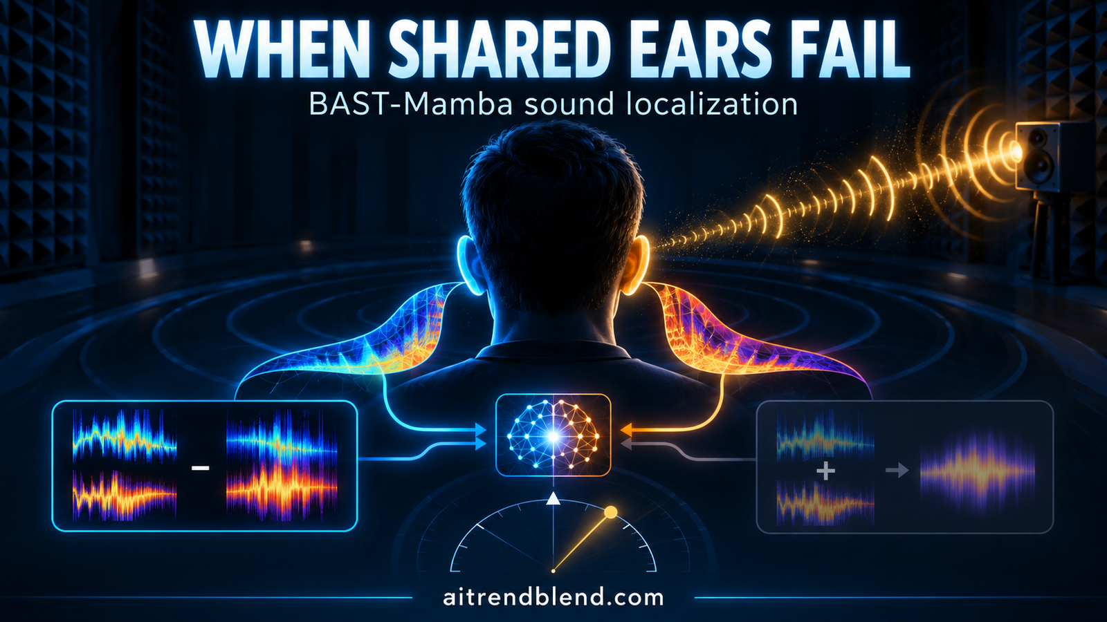
- BAST-Mamba feeds left and right ear spectrograms through separate encoders, fuses them with concatenation, addition, or subtraction, then predicts a 2D azimuth coordinate through a center encoder.
- The best configuration, MambaVision backbone, shared encoder weights, subtraction fusion, and a hybrid loss, reaches an angular distance of 0.89 degrees and a mean squared error of 0.0004.
- Sharing weights between the left and right encoders while fusing with simple addition breaks the model across all three tested backbones, pushing angular error above 10 degrees, worse than the paper’s own single stream baselines that ignore interaural cues entirely.
- Training on both anechoic and reverberant rooms together generalizes far better than training on either alone, which fails badly when tested in the other environment.
- Grad-CAM analysis shows the model’s attention concentrates in the 2 to 3 kHz and 5.5 to 6.5 kHz bands, matching frequency ranges known from human auditory neuroscience to carry strong interaural level cues.
- The system currently predicts only a flat 2D azimuth at a fixed distance, with no elevation and no tested adaptation to unfamiliar rooms.
The problem with teaching a machine to point at sound
Human listeners localize sound almost entirely from two cues, the tiny time gap between a sound reaching one ear before the other, and the level difference caused by the head blocking sound from the far ear. Prior deep learning attempts at this task fall into two camps. Convolutional networks are good at picking up local spectral texture but struggle to connect information spread far apart in a spectrogram, which matters because interaural cues can span a wide frequency range. Vision inspired Transformers handle that long range dependency well, yet almost none of the existing audio Transformer work builds in an explicit two ear structure the way biological hearing does.
A prior model called NI-CNN, from two of this paper’s own co-authors, tried to close that gap by processing each ear through separate convolutional layers before combining them, mimicking the brainstem structures that first merge signals from both cochleas. It worked, but its convolutional layers still could not model long range spectral relationships, and it depended on a cochlear preprocessing step rather than learning straight from raw audio.
BAST-Mamba is the authors’ attempt to keep NI-CNN’s dual ear structure while swapping convolution for Transformer style backbones, testing three candidates, the original Vision Transformer, the windowed Swin Transformer, and MambaVision, a newer hybrid that pairs a state space model mixer with attention. The paper is explicit that its goal is not just a leaderboard win but a closer functional match to the actual human auditory pathway, and several of its later experiments are framed around comparing model behavior to known human localization quirks.
How the three ear model actually works
The architecture has three encoders rather than the usual one or two. A spectrogram from the left ear and one from the right ear are each cut into overlapping patches, embedded, and passed through their own left and right encoder stacks, exactly as a standard Vision Transformer would treat two separate images. Each encoder can be built from ViT blocks, Swin blocks, or MambaVision blocks, and the paper tests all three.
The outputs of the left and right encoders are then combined by one of three interaural integration methods, meant to echo the way the human olivary nucleus merges binaural input. Concatenation stacks both feature maps along the channel dimension without discarding anything. Addition sums them, matching cues but also averaging away differences. Subtraction computes the right ear output minus the left ear output, which is the closest analog to how the lateral superior olive actually encodes level differences, combining excitatory input from one ear with inhibitory input from the other.
Whatever the fusion method produces feeds into a third encoder, the center encoder, built from the same backbone family as the left and right encoders. Its output is average pooled across all patches and passed through a single linear layer with no activation function, so the model’s predicted coordinate can land anywhere on the 2D plane rather than being squeezed into a bounded range.
Two ways to wire the ears together
A second design axis sits underneath all of this. The left and right encoders can either share the exact same weights, called the SP or shared parameter configuration, or be trained completely independently, called NSP. Sharing weights halves the number of parameters devoted to the two side encoders and forces the model to treat both ears with an identical function, which is architecturally elegant and mirrors the idea that a human auditory system does not literally grow two different processing modules for two ears. Independent weights give up that elegance for the freedom to let each side specialize.
Training with two kinds of error at once
The loss function matters as much as the architecture here. Plain mean squared error pushes predicted coordinates toward the true coordinates in Euclidean space, but it can tolerate a prediction that points in roughly the right direction while landing at the wrong distance from the origin. Angular distance loss fixes that by measuring only the angle between predicted and true direction vectors, ignoring magnitude entirely.
Used alone, angular distance loss places no constraint on how far from the origin a prediction sits, which the paper’s own results confirm produces unstable coordinate magnitudes in some configurations. The hybrid loss the authors settle on is a convex mix of both, keeping the orientation sensitivity of angular distance while using mean squared error to stop the model from drifting into degenerate solutions that get the direction right and everything else wrong.
The headline numbers, and where they come from
Training used 4600 real world sounds spatialized to 36 azimuth positions, run through both an anechoic simulation and a reverberant room impulse response recorded in a real lecture hall, producing 331200 training samples and a fully held out test set of 28800 samples from 400 new sound files. Every model was compared against a plain three layer CNN with no binaural structure at all, the earlier NI-CNN in two input variants, and FAViT, a prior audio Vision Transformer without an explicit dual ear design.
| Model | Angular distance ↓ | Mean squared error ↓ |
|---|---|---|
| CNN, single stream | 3.09° (hybrid loss) | 0.010 |
| FAViT, single stream | 3.73° (hybrid loss) | 0.015 |
| NI-CNN* (best fusion) | 1.85° | 0.031 |
| BAST-Mamba-NSP (best fusion) | 1.31° | 0.002 |
| BAST-Mamba-SP, subtraction, hybrid loss | 0.89° | 0.0004 |
That final row is a genuinely large improvement, more than a 75 percent drop in angular error against the strongest CNN baseline and a 90 percent drop in mean squared error. Across all three backbones, subtraction based fusion consistently produced the lowest errors, which the authors connect directly to the lateral superior olive’s own subtractive encoding of level differences, a nice case of a design choice motivated by neuroscience actually paying off in the numbers rather than just sounding good in the introduction.
The failure mode the paper reports but does not dwell on
Here is the part worth sitting with. Look at what happens to the shared parameter models specifically when they are fused with addition instead of subtraction or concatenation.
| Model, shared parameters | Fusion | Angular distance, hybrid loss ↓ |
|---|---|---|
| BAST-ViT-SP | Addition | 5.72° |
| BAST-Swin-SP | Addition | 9.46° |
| BAST-Mamba-SP | Addition | 10.42° |
| BAST-Mamba-SP | Subtraction | 0.89° |
Every single shared parameter model, regardless of whether its backbone is ViT, Swin, or MambaVision, gets dramatically worse the moment addition replaces subtraction or concatenation as the fusion method. The worst of the three, BAST-Mamba-SP with addition trained on pure angular distance loss, reaches 21.98 degrees. Set that against the plain single stream CNN from the baseline table, a model that never even sees two separate ears, which manages 3.09 to 3.90 degrees depending on loss function. A shared weight, addition fused BAST variant is worse at localizing sound than a model architecture that throws away the entire binaural signal and looks at one channel.
The paper offers a tidy explanation, and it is a correct one as far as it goes. When both encoders share identical weights, they tend to produce highly similar feature representations for similar input, so adding those two similar signals together mostly reinforces them rather than exposing the difference that actually carries spatial information. Independent encoders, even without any explicit constraint to do so, drift into different representations during training, so their sum still retains enough disparity for the center encoder to work with. That explanation is consistent with why NSP addition models perform reasonably, matching subtraction closely in that configuration, at 1.45 degrees against 1.31 degrees for BAST-Mamba-NSP.
What the paper does not spell out is how total the shared weight addition failure is, or that it repeats identically across all three backbone families tested. That consistency is itself informative. It rules out an implementation quirk specific to one architecture and points instead to a structural interaction between parameter sharing and additive fusion that any team building a similarly efficient dual stream audio model should expect to hit, not something to discover by accident during their own ablations.
A second fragility, this time about rooms rather than ears
The paper runs a separate experiment training its best configuration, BAST-Mamba-SP with subtraction and hybrid loss, on only anechoic data, only reverberant data, or a pooled mix of both, then testing on each environment.
| Trained on | Tested on | Angular distance ↓ |
|---|---|---|
| Anechoic only | Anechoic | 0.90° |
| Anechoic only | Reverberant | 23.73° |
| Reverberant only | Anechoic | 16.75° |
| Reverberant only | Reverberant | 1.11° |
| Both, pooled | Anechoic | 0.74° |
| Both, pooled | Reverberant | 1.03° |
A model trained on a clean, echo free room and then asked to localize sound in a real reverberant lecture hall is not merely a little worse, it is roughly 26 times worse than the same model trained and tested on matched conditions. The reverse direction is nearly as bad. Only once both acoustic conditions appear during training does the model become genuinely robust to either one, and doing so does not cost it anything relative to environment matched training, the pooled model actually edges out the anechoic only model even on the anechoic test set. That is a meaningful finding for deployment. A model this brittle to acoustic mismatch has effectively no real world value unless its training data spans the range of rooms it will ever be asked to work in, and the paper’s own tested range covers exactly two acoustic conditions.
What the frequency focus analysis adds
Beyond raw accuracy, the authors run Grad-CAM on the trained models to see which frequency bands the network actually attends to, then correlate that attention with localization error on a per frequency basis. The model consistently concentrates on the 2 to 3 kHz and 5.5 to 6.5 kHz bands, largely ignoring anything below 1.5 kHz. Only the lower of those two bands showed a statistically significant relationship with accuracy, a negative correlation of roughly negative 0.65, meaning more attention there tracked with lower error. Attention in the higher band did not significantly predict accuracy on its own, despite the model spending comparable attention there, and a narrow band around 6.5 to 7 kHz showed the opposite pattern, where more focus modestly predicted higher error.
That distinction matters because it is easy to read a frequency focus plot as evidence that every peak in the curve is doing useful work. Here the statistics say only one of the two major peaks is demonstrably linked to accuracy, and the model may be spending attention on the second band for reasons that do not directly help azimuth prediction, at least not in a way this analysis could detect.
Honest limits of the system as published
The authors are direct about scope. BAST-Mamba predicts a flat 2D azimuth at one fixed distance from the listener, not elevation or full 3D position, and it has been tested on exactly two simulated acoustic environments rather than a wide sample of real rooms. There is no online adaptation, so a deployed model cannot adjust itself if the acoustic environment drifts from what it saw in training, which the environment generalization table above suggests would be a serious problem if it happened. The noise robustness experiments cover synthetic Gaussian noise only, not the more structured interference of overlapping speech or mechanical hum that a real environment would introduce.
What this means if you are building something similar
For a team designing a dual stream audio model, three practical lessons come out of this reading. First, if parameter efficiency through weight sharing is a design goal, pair it with subtraction or concatenation based fusion rather than addition, since the paper’s numbers show that combination is not a minor tradeoff but a total failure across backbone types. Second, treat acoustic environment diversity in training data as load bearing rather than optional, given how sharply performance collapses under environment mismatch even when the core architecture and loss function stay identical. Third, when publishing a Grad-CAM or attention style interpretability figure, pair every visually prominent focus region with a statistical test against the outcome metric, because this paper’s own analysis shows one of its two headline frequency bands does not actually correlate with accuracy despite looking equally important in the raw attention plot.
Where the authors say this goes next
The paper’s stated next steps are modest and specific rather than sweeping. Extending the model to full 3D localization including elevation, testing against a wider and more realistic range of noise types beyond synthetic Gaussian noise, and adding some form of lightweight online adaptation so a deployed model could adjust to a new room without full retraining. None of these are underway yet in the paper itself, they are stated as future work, and the released code covers only the 2D anechoic and reverberant setup described here.
Limitations of this analysis
This reading relies entirely on the tables and figures the authors published, without independently rerunning their training pipeline or accessing their raw per sample predictions. The shared weight addition failure is drawn directly from the paper’s own Table 1 across three backbones, but confirming the mechanism the authors propose, that shared encoders converge to similar representations that addition then reinforces rather than exposes, would require inspecting the actual learned features, which the paper does not report and this article does not attempt to reconstruct. The frequency correlation figures are likewise taken as reported, and this article adds no independent statistical test of its own beyond what the authors already computed.
Reimplementing the fusion comparison on a toy model
The following is a compact PyTorch script that builds a small dual encoder Transformer, similar in spirit to the paper’s left and right encoder design, and compares shared versus independent encoder weights under addition and subtraction fusion on synthetic data. It is not the authors’ code, it is a minimal reimplementation meant to check that the interaction described above, shared weights making addition fusion collapse toward a near zero signal, actually shows up in a toy setting.
import torch
import torch.nn as nn
import torch.nn.functional as F

# --- a minimal patch based encoder, standing in for the ViT/Swin/MambaVision blocks --

class TinyEncoder(nn.Module):
    def __init__(self, dim=32, n_patches=16, n_layers=2):
        super().__init__()
        self.pos = nn.Parameter(torch.randn(1, n_patches, dim) * 0.02)
        self.layers = nn.ModuleList([
            nn.TransformerEncoderLayer(d_model=dim, nhead=4, dim_feedforward=dim * 2, batch_first=True)
            for _ in range(n_layers)
        ])

    def forward(self, patches):
        x = patches + self.pos
        for layer in self.layers:
            x = layer(x)
        return x

# --- the center encoder and prediction head, shared by every configuration --------

class CenterHead(nn.Module):
    def __init__(self, dim=32, in_dim=None, n_patches=16):
        super().__init__()
        in_dim = in_dim or dim
        self.center = TinyEncoder(dim=in_dim, n_patches=n_patches)
        self.out = nn.Linear(in_dim, 2)

    def forward(self, fused):
        z = self.center(fused)
        pooled = z.mean(dim=1)
        return self.out(pooled)

# --- one full dual ear model, either shared (SP) or independent (NSP) encoders ----

class DualEarModel(nn.Module):
    def __init__(self, dim=32, n_patches=16, shared=True, fusion="addition"):
        super().__init__()
        self.shared = shared
        self.fusion = fusion
        self.left = TinyEncoder(dim=dim, n_patches=n_patches)
        self.right = self.left if shared else TinyEncoder(dim=dim, n_patches=n_patches)
        fused_dim = dim * 2 if fusion == "concat" else dim
        self.head = CenterHead(dim=dim, in_dim=fused_dim, n_patches=n_patches)

    def forward(self, left_patch, right_patch):
        zl = self.left(left_patch)
        zr = self.right(right_patch)
        if self.fusion == "addition":
            fused = zl + zr
        elif self.fusion == "subtraction":
            fused = zr - zl
        else:
            fused = torch.cat([zl, zr], dim=-1)
        return self.head(fused)

# --- hybrid loss, mean squared error plus angular distance -----------------------

def hybrid_loss(pred, target, alpha=0.5, eps=1e-6):
    mse = F.mse_loss(pred, target)
    cos = F.cosine_similarity(pred, target, dim=-1, eps=eps).clamp(-1 + eps, 1 - eps)
    ad = torch.acos(cos).mean() / torch.pi
    return alpha * mse + (1 - alpha) * ad, mse.item(), ad.item()

# --- smoke test, mirroring the paper's shared weight plus addition comparison ----

def smoke_test():
    torch.manual_seed(0)
    dim, n_patches, batch = 32, 16, 64

    # synthetic left and right patch embeddings that differ mainly through a small
    # interaural offset, standing in for a real ILD/ITD cue
    target_angle = torch.rand(batch) * 2 * torch.pi
    target = torch.stack([torch.cos(target_angle), torch.sin(target_angle)], dim=-1)

    base = torch.randn(batch, n_patches, dim)
    ild_cue = target_angle.view(-1, 1, 1) * 0.05
    left_patch = base - ild_cue
    right_patch = base + ild_cue

    results = {}
    for shared in [True, False]:
        for fusion in ["addition", "subtraction"]:
            model = DualEarModel(dim=dim, n_patches=n_patches, shared=shared, fusion=fusion)
            opt = torch.optim.Adam(model.parameters(), lr=1e-3)
            for step in range(200):
                opt.zero_grad()
                pred = model(left_patch, right_patch)
                loss, mse, ad = hybrid_loss(pred, target)
                loss.backward()
                opt.step()
            results[(shared, fusion)] = (mse, ad)
            print(f"shared={shared} fusion={fusion} final mse={mse:.4f} final ad={ad:.4f}")

    # the qualitative claim we are checking, shared weights hurt addition fusion
    # far more than it hurts subtraction fusion
    shared_add_ad = results[(True, "addition")][1]
    shared_sub_ad = results[(True, "subtraction")][1]
    indep_add_ad = results[(False, "addition")][1]
    print("shared addition worse than shared subtraction:", shared_add_ad > shared_sub_ad)
    print("shared addition worse than independent addition:", shared_add_ad > indep_add_ad)
    print("smoke test passed")

if __name__ == "__main__":
    smoke_test()
Bringing it together
BAST-Mamba’s core achievement holds up under scrutiny. Building a genuinely three encoder architecture, left, right, and center, around Transformer backbones rather than convolution, and letting the fusion method and parameter sharing choice vary independently, produces a model that beats every tested baseline by a wide margin and does so while echoing a real piece of auditory neuroscience, the subtractive computation performed by the lateral superior olive. The 0.89 degree angular error is a legitimate result, not an artifact of an unfair comparison.
The conceptual shift worth carrying forward is that biological structure, here an explicit two ear architecture with a biologically motivated fusion rule, can outperform simply throwing a bigger attention mechanism at the raw problem. That is a useful data point for anyone working at the intersection of neuroscience inspired architecture design and general purpose Transformer backbones, and it should transfer to other paired sensor problems beyond hearing, anywhere a system genuinely has two correlated but distinct input streams.
Where this article pushes back is on how completely the paper’s efficiency story depends on choosing the right fusion method. The abstract highlights the shared parameter model as the best performer, which is true only for subtraction fusion. Pair that same efficient architecture with addition, the most naive fusion choice a less careful implementation might reach for first, and the result is worse than not modeling two ears at all. That is not a footnote buried in an ablation, it repeats identically across three different backbone families, which means it is a property of the shared weight plus addition combination itself rather than a quirk of any one architecture.
Honest remaining limitations sit alongside that finding. The system has only ever seen two acoustic environments, predicts azimuth alone with no elevation or distance, and has no tested mechanism for adapting to a new room without retraining, a gap the environment generalization table above suggests would matter a great deal in practice. None of this undercuts the central architectural idea, but a team evaluating this approach for a real deployment should treat the reported numbers as describing a controlled, two room benchmark rather than open ended real world performance.
Future directions the authors name, full 3D localization, broader noise modeling, and lightweight online adaptation, all point at the same underlying gap, that the model’s excellent numbers currently come from training and testing within a narrow, well characterized acoustic world. Closing that gap, more than any further architecture search among Transformer backbones, looks like the more consequential next step for turning this into something that works outside a lab recorded lecture hall.
Pingback: Revolutionizing Lower Limb Motor Imagery Classification: A 3D-Attention MSC-T3AM Transformer Model with Knowledge Distillation - aitrendblend.com