
Key points
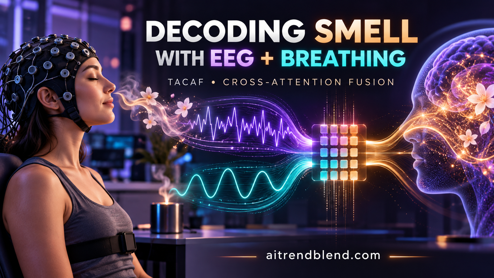
- TACAF is a multimodal deep learning model from Nanyang Technological University and Wilmar International that decodes pleasant versus unpleasant odor responses from EEG and breathing signals together.
- Instead of choosing a fixed time window by hand, the model uses wavelet decomposition to pick a segmentation length automatically based on the highest frequency band it cares about.
- A Temporal Token Semantic Alignment module converts the raw breathing signal into tokens that line up in time with the EEG tokens, so the two streams can actually be compared.
- A cross attention layer fuses breathing into EEG, and this fusion strategy beat simple summing, averaging, and concatenation in head to head tests.
- TACAF reached 71.24 percent accuracy within subject and 61.80 percent accuracy across subjects, ahead of ten established EEG and olfactory decoding baselines.
- Breathing alone barely beat chance at 51 to 52 percent, yet adding it to EEG lifted accuracy by more than three points, showing it guides the model rather than leaking the answer on its own.
This article explains a piece of published neuroscience and engineering research. It is not medical advice, diagnosis, or treatment.
Nothing here should be used to interpret your own brain activity, breathing patterns, or sense of smell. If you have concerns about your sense of smell or neurological health, talk with a qualified physician.
Why teaching a computer to smell through your brainwaves is genuinely hard
Smell sits close to memory and emotion in a way most other senses do not, a link the paper traces back through decades of neuroscience on how the olfactory bulb feeds almost directly into the limbic system. That closeness is exactly why researchers want to read it out of brain activity in the first place. A reliable way to decode whether an odor registers as pleasant or unpleasant could eventually support work in food product development or in understanding conditions where smell and mood interact, the kind of application the paper gestures toward without claiming to have built.
The trouble is that scalp EEG, while it offers good temporal resolution and covers many regions at once, is a messy signal to mine for something as fleeting as a whiff of scent. Earlier work leaned on hand crafted features such as power spectral density across frequency bands or differential entropy, approaches that need a domain expert to decide which bands and which statistics matter before a classifier ever sees the data. More recent deep learning models, from DeepConvNet and EEGNet built for general brain computer interfaces to purpose built olfactory networks like TESANet, TASA, FBANet, and EEG-LGFNet, moved toward learning those features directly from raw or lightly processed EEG. Even so, the paper identifies two gaps none of that prior work closed.
Two problems that kept getting worked around instead of solved
The first gap is temporal segmentation. Almost every prior olfactory EEG model chops the signal into time windows using a fixed, empirically chosen length, a number someone picked because it worked reasonably well rather than because the signal itself demanded it. That risks smoothing over exactly the subtle, fast moving patterns an odor response produces.
The second gap is breathing. Inhalation timing and depth are known to shape how an odor is perceived, since molecules need to migrate through the nasal cavity at a pace set by the breath itself, yet almost no prior olfactory EEG model actually collects and uses a breathing signal. TASA, one of the paper’s own closest predecessors, found that its learned attention weights happened to correlate with breathing phase even though breathing was never fed into the model, a hint that the information was there for the taking and nobody had taken it.
TACAF, short for Token Alignment and Cross Attention Fusion network, is built to close both gaps at once, letting the wavelet transform choose the time windows and letting a dedicated alignment module bring breathing into the same representation space as the EEG.
Letting the wavelet transform pick the time window instead of guessing
Rather than slicing EEG into arbitrary chunks, TACAF runs a multi level wavelet decomposition on the raw signal using the simplest possible mother wavelet, the Daubechies-1 wavelet, across seven decomposition levels. From that decomposition it keeps the coefficients for five frequency bands that map onto the classic EEG ranges, 0 to 4 Hz, 4 to 8 Hz, 8 to 16 Hz, 16 to 32 Hz, and 32 to 63 Hz.
Wavelet transforms carry a built in time frequency trade off, finer time resolution at higher frequencies and coarser time resolution at lower ones, and TACAF leans into that property rather than fighting it. The segment length is set by the highest frequency band it uses, 32 to 63 Hz, since that band naturally yields the shortest, most temporally precise segments. The lower frequency bands, which the wavelet transform naturally represents with longer segments, get their coefficients repeated so every band ends up sharing the same number of time segments.
The result is a tensor X_WT with shape S by F by C, where S is the number of time windows the wavelet transform itself decided on, F is the five frequency bands, and C is the EEG channel count. Every one of those time segments carries frequency content from 0 up to 63 Hz, the range that matters for EEG analysis.
Turning wavelet features into tokens a transformer can read
That time frequency tensor still needs to become something an attention mechanism can operate on. A spatial filtering module handles the channel dimension first, two stacked blocks of fully connected layers that project the channel count down through an intermediate size to a final output size, each block followed by batch normalization and an ELU activation.
In the paper’s implementation the two linear layers output sizes of 30 and then 10, so the final channel dimension lands at 10. The result is flattened across the frequency and channel dimensions into a single feature vector per time segment.
That flattened representation then passes through standard multi head self attention, the same mechanism that powers most modern transformer models, computed per head as scaled dot product attention over the query, key, and value projections of the flattened features, then concatenated across heads and linearly projected to the final attention output.
Two attention heads are used in the paper’s configuration, with an output dimension of 128. What this attention layer is actually learning is the intercorrelation between the wavelet chosen time segments themselves, effectively how one moment of the odor response relates to another moment, which is the core temporal dynamics signal the whole architecture is built around.
Teaching breathing to speak the same language as EEG
A raw breathing trace and a stack of EEG attention tokens do not naturally line up. The breathing signal is a single continuous channel sampled at the same 1000 Hz as the EEG, with none of the frequency band structure the wavelet transform imposed on the brain data. The Temporal Token Semantic Alignment module, TTSA for short, exists to close that gap by reshaping breathing into the same number of tokens the EEG side produced.
TTSA borrows the spirit of wavelet decomposition without literally running one. Each of its layers is a 1D convolution with a kernel sized to match the mother wavelet, a stride of 2, batch normalization, and an ELU activation, which halves the sequence length at every layer the same way one level of wavelet decomposition would.
Four such layers are stacked, taking the single input channel up through H over 8, H over 4, H over 2, and finally H channels, where H is 128 to match the EEG side. After the last layer the breathing representation is reshaped to the same S by H shape the EEG attention module produced, meaning every breathing token and every EEG token now correspond to the same point in the trial’s timeline.
Fusing brain and breath through cross attention
With both modalities expressed as aligned token sequences, TACAF fuses them with cross attention rather than a simpler merge like concatenation. The breathing tokens generate the query, while the EEG tokens generate both the key and the value, so the fused representation is explicitly built by asking what in the EEG sequence each breathing moment should attend to.
The fusion output dimension D is 256, and the fused representation flows into a single fully connected layer with a softmax to produce the pleasant versus unpleasant prediction, trained with ordinary cross entropy loss and the Adam optimizer.
| Stage | Operation | Output shape |
|---|---|---|
| EEG modality | Wavelet decomposition and interpolation | S by F by C |
| EEG modality | Spatial filtering across channels | S by F by C_out |
| EEG modality | Flatten and multi head self attention | S by H |
| Breathing modality | TTSA and reshape | S by H |
| Fusion | Cross attention | S by D |
| Classification | Flatten, linear, softmax | Number of classes |
How the study was actually run
Twenty subjects took part, averaging 31.95 years old with a standard deviation of 8.97 years, all recruited from Wilmar International in Singapore, where the data collection also took place. The study was approved by the Nanyang Technological University Institutional Review Board under protocol IRB-2023-378, and every participant gave written consent. Participants were non smokers, right handed, free of any history of major neurological disease, not pregnant or breastfeeding, and screened with the extended Sniffin’ Sticks test, a standard clinical tool covering odor threshold, discrimination, and identification. Only people scoring above 30.5 on the composite TDI measure, indicating normal olfactory function, were included, and everyone was asked to avoid strongly flavored food and perfume on the day of testing.
Odor delivery used a Burghart OL023 research olfactometer running a constant 8 liter per minute flow at 36 degrees Celsius. Two odorants were used, 2-Phenyl-Ethanol diluted to 0.1 percent as the pleasant stimulus and Diethyl Disulfide diluted to 0.25 percent as the unpleasant one, both carried in diethyl phthalate. EEG came from a 64 channel actiCHamp system, with breathing captured by a respiration belt, everything sampled at 1000 Hz and time synchronized, and four of the sixty four channels were reserved for eye movement monitoring rather than EEG proper.
Each trial followed a fixed rhythm shown in the paper’s trial diagram. The system waited for the participant to inhale, released one of the two odors for 4 seconds timed to match a full respiration cycle at a typical 15 breaths per minute, then gave a 10 second rest before the next trial, a gap chosen because it produced a cleaner signal to noise ratio in earlier chemosensory research. Fifty trials made up one session, and four sessions per participant added up to 200 trials total, with odors randomized and balanced between pleasant and unpleasant. The first 100 trials were used to build and evaluate the classification model, and the second 100 trials were kept as an entirely separate set for studying whether performance changed with repeated odor exposure.
Preprocessing used Independent Component Analysis for artifact removal and a 0.5 to 64 Hz bandpass filter, implemented in the MNE Python package, with every trial visually checked before inclusion. Each trial was epoched from 0 to 4 seconds relative to the start of odor release. Two evaluation protocols were used throughout, Subject Dependent testing with nested trial wise 10 fold cross validation for each individual subject, and Leave One Subject Out testing where the model trains on 19 subjects and is tested on the twentieth, repeated so every subject serves as the held out test once. A grid search over learning rates from 1 times 10 to the negative 5 up to 1 times 10 to the negative 3 picked the best setting on a held out validation split before final testing.
How well TACAF actually decoded pleasant from unpleasant
TACAF reached 71.24 percent accuracy under the Subject Dependent protocol and 61.80 percent under Leave One Subject Out, and it posted the lowest standard deviation of any tested method under both protocols, a sign of more consistent performance across folds and subjects rather than just a higher average.
| Method | Subject Dependent | Leave One Subject Out |
|---|---|---|
| FBCSP | 57.38% | 53.21% |
| DeepConvNet | 60.00% | 55.45% |
| EEGNet | 62.91% | 55.49% |
| CRAM | 65.55% | 56.17% |
| 3DCNN-BiLSTM | 66.05% | 56.40% |
| FBANet | 65.93% | 57.50% |
| EEG-LGFNet | 64.12% | 57.33% |
| TESANet | 66.21% | 57.08% |
| EEG-Deformer | 65.24% | 56.78% |
| TASA | 67.07% | 57.59% |
| TACAF (proposed) | 71.24% | 61.80% |
Statistical testing backs the gap up. Against every one of the ten baselines the improvement is significant, with p values below 0.01 in every case and below 0.0001 against several of them, including the general purpose FBCSP, DeepConvNet, and EEGNet models. The paper’s own reading of why certain baselines fall short is worth sitting with. Plain convolutional models like EEGNet and DeepConvNet lag behind attention based methods, which the authors attribute to weaker temporal dynamics modeling. CRAM uses attention but not self attention across time segments, limiting how well it captures intercorrelation between moments. EEG-Deformer models both coarse and fine grained temporal features but still relies on fixed, non adaptive time windows. The purpose built olfactory models FBANet, EEG-LGFNet, TESANet, and TASA all do reasonably well, and TASA in particular, the paper’s own direct predecessor, comes closest to TACAF, which makes sense given how directly TACAF builds on its lineage.
Smell fades with repetition, and the model noticed
Because the study collected 200 trials per person across four sessions, the researchers could ask whether decoding accuracy held steady over that stretch or degraded, a question tied to a well known phenomenon called olfactory adaptation, where repeated or prolonged exposure to an odor reduces the nervous system’s sensitivity to it.
| Trial range | Subject Dependent | Leave One Subject Out |
|---|---|---|
| Trials 1 to 100 | 71.24% | 61.80% |
| Trials 101 to 200 | 62.03% | 54.11% |
| All 200 trials combined | 65.70% | 55.39% |
The first 100 trials outperformed the second 100 by 9.21 points under Subject Dependent testing and 7.69 points under Leave One Subject Out, and even beat the combined 200 trial setting by more than five points in both protocols. The authors connect this directly to olfactory adaptation, which is known to occur at both the brain level and the olfactory epithelium itself, and note that adaptation can shift reaction time and the temporal shape of the response, which would explain why a model trained across the full stretch of trials performs worse than one trained only on the earlier, less adapted trials.
Cross attention beat every simpler way of combining the two signals
To justify choosing cross attention over a simpler merge, the authors tested summing the two modalities, averaging them, and concatenating them, all as direct substitutes for the cross attention fusion layer.
| Fusion method | Subject Dependent | Leave One Subject Out |
|---|---|---|
| Sum | 69.10% | 56.95% |
| Average | 69.25% | 56.80% |
| Concatenation | 68.11% | 57.65% |
| Cross attention (proposed) | 71.24% | 61.80% |
Sum and average treat both modalities as equally weighted contributors regardless of what is actually happening at a given moment, and concatenation simply places the two feature vectors side by side without modeling how they relate. Cross attention is the only one of the four that explicitly computes intercorrelation between EEG and breathing tokens, letting breathing information actively steer which parts of the EEG sequence the model leans on, and the Leave One Subject Out gap in particular, more than four points over the next best fusion strategy, suggests that steering effect matters even more when generalizing to a new person.
Inhaling versus exhaling barely matters on its own
Since a full trial spans one complete breath, the researchers also split each 4 second window into an inhale half from 0 to 2 seconds and an exhale half from 2 to 4 seconds, treating each as its own independent dataset.
| Window | Subject Dependent | Leave One Subject Out |
|---|---|---|
| 0 to 2 seconds, inhale phase | 66.73% | 56.95% |
| 2 to 4 seconds, exhale phase | 66.01% | 55.65% |
| 0 to 4 seconds, full trial | 71.24% | 61.80% |
Inhale edged out exhale by just 0.72 points under Subject Dependent testing and 1.30 points under Leave One Subject Out, a small enough gap that the authors read it as evidence the odor response is a continuous process rather than something concentrated in one breathing phase, with useful discriminative information spread across the whole respiration cycle. That reading also explains why the full trial beats either half by roughly five points, since it captures both halves of that continuous signal rather than throwing part of it away.
Checking whether the model is secretly just reading breathing patterns
A fair question for any multimodal result like this is whether the gain from adding breathing is real neural signal or just an artifact of people unconsciously changing how they breathe when a smell is unpleasant. The authors ran a direct modality ablation to check.
| Modality used | Subject Dependent | Leave One Subject Out |
|---|---|---|
| EEG only | 67.95% | 58.45% |
| Breathing only | 51.25% | 52.30% |
| EEG plus breathing, full model | 71.24% | 61.80% |
Breathing on its own sits right around chance level for a balanced two class problem, meaning the respiration trace by itself carries essentially no information about whether the odor was pleasant or not. That is a reassuring result rather than a disappointing one, because it means the roughly three point boost the full model gets over EEG alone cannot be explained by subjects simply breathing differently when a smell is unpleasant. Instead, breathing appears to work as a guide that helps the model extract more discriminative structure from the EEG signal itself, consistent with the physiological argument that inhalation timing shapes how odor molecules reach olfactory receptors in the first place.
The results indicate that our collected breathing signal alone is unable to differentiate between the two classes. However, when the breathing signal interacts with EEG, the performance increases, suggesting that the breathing signal alone does not provide sufficient information to discriminate between the two classes, but it guides the EEG data to learn more discriminative features. The paper’s own discussion of the modality ablation, Section 6
A model that stays small while it wins
Accuracy gains often come with a computational tax, so the authors also compared parameter counts and multiply accumulate operations, MACs, across every method. TACAF landed at roughly 59.11 million MACs and 254 thousand parameters, a genuinely compact footprint next to EEG-LGFNet’s 1,868 million MACs for noticeably lower accuracy, or 3DCNN-BiLSTM’s 7,244 thousand parameters despite using far fewer MACs than TACAF. Smaller models like FBANet and EEGNet trade away some accuracy in exchange for that lighter footprint, while TACAF manages to sit near the efficient end of the field and still post the best accuracy overall, a combination the authors frame as practical for real olfactory EEG decoding rather than purely a benchmark exercise.
Where in the brain the model is actually looking
To make the network’s decisions somewhat interpretable, the authors generated saliency maps along the EEG channel axis and plotted them as scalp topology maps. Frontal and temporal regions stood out as the most informative for classifying odor pleasantness, a pattern the paper ties to a body of earlier work linking those same regions to emotion valence processing more broadly, which lines up with how closely olfaction and emotion are wired together in the brain. That overlap is offered as evidence the network has learned something neurophysiologically sensible rather than an arbitrary pattern that merely happens to separate the two classes in this particular dataset.
The clinical translation gap
It is worth being precise about what this study does and does not show. Twenty healthy, olfactorily normal adults recruited from a single company in Singapore, tested in a controlled lab with a research grade olfactometer delivering two specific, carefully dosed odorants, is a long way from a deployable tool for assessing anyone’s sense of smell in a clinic or at home. The paper itself frames its contribution around decoding performance and neuroscience insight, not around any diagnostic or therapeutic claim, and nothing in the results should be read as evidence that this system can detect smell disorders, mood conditions, or any other health state.
The gap between Subject Dependent and Leave One Subject Out accuracy, 71.24 percent falling to 61.80 percent, is itself a meaningful signal about how far this is from a plug and play tool. A model that performs noticeably better when it has already seen a person’s own data than when meeting a new person for the first time is a common and expected pattern in EEG based brain computer interfaces, but it is also exactly the kind of gap that would need to close substantially before a system like this could be handed to a new user without individual calibration.
Honest limitations
The sample size is small by the standards of clinical research, twenty participants, even though the nested cross validation and nineteen fold Leave One Subject Out protocol squeeze a reasonable amount of evaluation out of that group. All twenty were recruited from a single employer, Wilmar International, which likely skews the sample toward working age adults in one geographic and occupational setting rather than a broad population, and the mean age of 31.95 years with a standard deviation of 8.97 years leaves both children and older adults entirely unrepresented, a population where olfactory function and EEG characteristics can both differ meaningfully.
The task itself is a binary one, distinguishing exactly two specific odorants at fixed concentrations, not the much larger and more continuous space of real world smells and intensities. Every participant also passed a Sniffin’ Sticks screening confirming normal olfactory function, meaning the study says nothing about how this approach would perform for someone with reduced or altered sense of smell, a population where a tool like this might eventually be most useful.
The authors themselves flag two further limitations directly. Olfactory adaptation, the phenomenon behind the drop in accuracy across trials, occurs at both the brain and the olfactory epithelium, and this study cannot separate those two contributions since it only records EEG rather than adding something like electro-olfactogram recordings at the epithelium itself. They also note that spatial and temporal dynamics were modeled somewhat separately in this architecture, spatial filtering first and temporal self attention second, and suggest a more joint spatiotemporal approach as a direction for future work rather than something already solved here.
Where this fits in the bigger picture
The specific accuracy numbers matter less than the two design principles the paper demonstrates. Letting a signal’s own frequency content decide its time segmentation, rather than picking a window length by hand, is a pattern that could transfer well beyond olfactory EEG to any brain computer interface task wrestling with how finely to slice a continuous signal. And the modality ablation showing breathing at chance level alone but genuinely useful once cross attended into EEG is a clean demonstration of how a weak, low information modality can still meaningfully improve a stronger one if the fusion mechanism is built to model the interaction rather than just average the two together. Both ideas seem likely to show up again in future multimodal physiological signal work, inside and outside olfaction research specifically.
Conclusion
TACAF earns its place in the olfactory EEG literature by solving two problems that the field had mostly worked around rather than fixed. Wavelet based automatic time window selection replaces the guesswork of fixed segmentation lengths, and the Temporal Token Semantic Alignment module finally gives breathing a real seat at the table alongside EEG rather than leaving it uncollected the way almost every prior olfactory decoding study did. The result is 71.24 percent accuracy within subject and 61.80 percent across subjects, ahead of ten established baselines with statistical significance behind nearly every comparison.
The conceptual shift worth carrying forward is treating time segmentation itself as something to learn from the signal’s own structure rather than a fixed preprocessing choice, paired with a fusion mechanism, cross attention, that is explicitly built to model how one modality should inform another rather than simply blending them. Both ideas are general enough to matter well outside olfactory neuroscience, anywhere a weaker physiological signal like breathing, heart rate, or skin conductance might sharpen a stronger one like EEG if it is aligned and fused with enough care.
None of that erases the real constraints on what this particular study shows. Twenty participants from one company, two odorants at fixed concentrations, and a meaningful accuracy drop when generalizing to a new person all mark this as an early, carefully executed research result rather than a system ready for deployment. The authors are candid about this themselves, right down to naming the joint spatiotemporal modeling gap and the unresolved question of where exactly, brain or epithelium, the observed olfactory adaptation is coming from.
Where this heads next seems reasonably clear from the paper’s own closing notes, adding electro-olfactogram recordings to separate brain level from epithelium level adaptation, exploring a more genuinely joint spatial and temporal architecture rather than the current two stage design, and presumably testing the approach on a larger and more demographically varied sample before any claim about generalizability beyond this one workplace cohort would be warranted.
For anyone building multimodal biosignal decoders more broadly, the lesson worth taking from TACAF is not really about smell specifically. It is that a secondary signal does not need to be independently informative to be worth collecting, as long as the fusion mechanism is designed to ask what one stream should tell you about another rather than just stacking them side by side.
Complete PyTorch implementation
The implementation below reconstructs the core pieces of TACAF, the wavelet based time window construction, the spatial filtering block, the multi head self attention module for EEG, the TTSA module for breathing, the cross attention fusion layer, and a runnable smoke test on random dummy data. Wavelet decomposition uses the PyWavelets library, referenced here as pywt.
# tacaf.py
# Reconstruction of the TACAF architecture described in
# "Decoding olfactory response from neurophysiological signal with
# a multimodal deep learning framework", Neural Networks 191 (2025) 107775.

import numpy as np
import pywt
import torch
import torch.nn as nn
import torch.nn.functional as F


def wavelet_time_windows(eeg, wavelet="db1", levels=7, bands=5):
    """Equation 1. Multi level wavelet decomposition of a single trial
    followed by interpolation so every frequency band shares the same
    number of time segments, matching the highest frequency band.
    eeg: numpy array of shape (C, T)."""
    c, t = eeg.shape
    coeffs_per_channel = []
    for ch in range(c):
        coeffs = pywt.wavedec(eeg[ch], wavelet, level=levels)
        # Keep the finest `bands` detail levels, matching 0-4, 4-8, 8-16,
        # 16-32, and 32-63 Hz as described in the paper.
        selected = coeffs[-bands:]
        target_len = len(selected[-1])
        interpolated = []
        for band in selected:
            repeat_factor = int(np.ceil(target_len / len(band)))
            band_rep = np.repeat(band, repeat_factor)[:target_len]
            interpolated.append(band_rep)
        coeffs_per_channel.append(np.stack(interpolated, axis=1))  # (S, F)

    # Stack across channels to get (S, F, C)
    x_wt = np.stack(coeffs_per_channel, axis=-1)
    return torch.tensor(x_wt, dtype=torch.float32)


class SpatialFilter(nn.Module):
    """Equation 2. Two stacked blocks projecting the channel dimension
    down to C_out, each a linear layer, batch norm, and ELU."""

    def __init__(self, c_in, c_mid=30, c_out=10):
        super().__init__()
        self.block1 = nn.Sequential(nn.Linear(c_in, c_mid), nn.BatchNorm1d(c_mid), nn.ELU())
        self.block2 = nn.Sequential(nn.Linear(c_mid, c_out), nn.BatchNorm1d(c_out), nn.ELU())

    def forward(self, x):
        # x: (batch, S, F, C) -> filtered along the C dimension
        b, s, f, c = x.shape
        x = x.view(b * s * f, c)
        x = self.block1(x)
        x = self.block2(x)
        return x.view(b, s, f, -1)


class MultiHeadSelfAttention(nn.Module):
    """Equations 4 and 5. Standard multi head self attention over the
    S wavelet derived time segments."""

    def __init__(self, dim_in, dim_out=128, num_heads=2):
        super().__init__()
        self.num_heads = num_heads
        self.head_dim = dim_out // num_heads
        self.q = nn.Linear(dim_in, dim_out)
        self.k = nn.Linear(dim_in, dim_out)
        self.v = nn.Linear(dim_in, dim_out)
        self.out_proj = nn.Linear(dim_out, dim_out)

    def forward(self, x):
        # x: (batch, S, F*C_out)
        b, s, _ = x.shape
        q = self.q(x).view(b, s, self.num_heads, self.head_dim).transpose(1, 2)
        k = self.k(x).view(b, s, self.num_heads, self.head_dim).transpose(1, 2)
        v = self.v(x).view(b, s, self.num_heads, self.head_dim).transpose(1, 2)

        scores = (q @ k.transpose(-2, -1)) / (self.head_dim ** 0.5)
        attn = F.softmax(scores, dim=-1)
        heads = attn @ v
        heads = heads.transpose(1, 2).reshape(b, s, -1)
        return self.out_proj(heads)


class TTSA(nn.Module):
    """Equation 6. Four 1D-CNN layers with stride 2, batch norm, and
    ELU, downsampling breathing to match the EEG token count."""

    def __init__(self, hidden_dim=128, kernel_size=2):
        super().__init__()
        dims = [1, hidden_dim // 8, hidden_dim // 4, hidden_dim // 2, hidden_dim]
        layers = []
        for i in range(4):
            layers.append(nn.Sequential(
                nn.Conv1d(dims[i], dims[i + 1], kernel_size=kernel_size, stride=2, padding=0),
                nn.BatchNorm1d(dims[i + 1]),
                nn.ELU(),
            ))
        self.layers = nn.ModuleList(layers)

    def forward(self, x):
        # x: (batch, 1, T)
        for layer in self.layers:
            x = layer(x)
        # x: (batch, H, S) -> reshape to (batch, S, H)
        return x.transpose(1, 2)


class CrossAttentionFusion(nn.Module):
    """Equations 7 and 8. Breathing tokens generate the query, EEG
    tokens generate the key and value."""

    def __init__(self, dim_in=128, dim_out=256, num_classes=2):
        super().__init__()
        self.q = nn.Linear(dim_in, dim_out)
        self.k = nn.Linear(dim_in, dim_out)
        self.v = nn.Linear(dim_in, dim_out)
        self.classifier = nn.Linear(dim_out, num_classes)
        self.dim_out = dim_out

    def forward(self, breathing_tokens, eeg_tokens):
        q_breath = self.q(breathing_tokens)
        k_eeg = self.k(eeg_tokens)
        v_eeg = self.v(eeg_tokens)

        scores = (q_breath @ k_eeg.transpose(-2, -1)) / (self.dim_out ** 0.5)
        attn = F.softmax(scores, dim=-1)
        fused = attn @ v_eeg

        logits = self.classifier(fused.mean(dim=1))
        return F.softmax(logits, dim=-1)


class TACAF(nn.Module):
    """Full Token Alignment and Cross Attention Fusion network."""

    def __init__(self, num_channels, num_bands=5, hidden_dim=128,
                 fusion_dim=256, num_classes=2):
        super().__init__()
        self.spatial_filter = SpatialFilter(num_channels, c_mid=30, c_out=10)
        self.eeg_attention = MultiHeadSelfAttention(
            dim_in=num_bands * 10, dim_out=hidden_dim, num_heads=2
        )
        self.ttsa = TTSA(hidden_dim=hidden_dim)
        self.fusion = CrossAttentionFusion(
            dim_in=hidden_dim, dim_out=fusion_dim, num_classes=num_classes
        )

    def forward(self, x_wt, x_breathing):
        # x_wt: (batch, S, F, C), x_breathing: (batch, 1, T)
        x_feature = self.spatial_filter(x_wt)
        b, s, f, c_out = x_feature.shape
        x_flat = x_feature.reshape(b, s, f * c_out)
        x_attention = self.eeg_attention(x_flat)

        x_feature_br = self.ttsa(x_breathing)
        # Align token counts in case of off by one rounding differences.
        min_len = min(x_attention.size(1), x_feature_br.size(1))
        x_attention = x_attention[:, :min_len]
        x_feature_br = x_feature_br[:, :min_len]

        return self.fusion(x_feature_br, x_attention)


def train_one_epoch(model, loader, optimizer, device):
    model.train()
    running_loss = 0.0
    for x_wt, x_breathing, labels in loader:
        x_wt, x_breathing, labels = x_wt.to(device), x_breathing.to(device), labels.to(device)
        optimizer.zero_grad()
        probs = model(x_wt, x_breathing)
        loss = F.nll_loss(torch.log(probs.clamp(min=1e-8)), labels)
        loss.backward()
        optimizer.step()
        running_loss += loss.item() * labels.size(0)
    return running_loss / len(loader.dataset)


@torch.no_grad()
def evaluate(model, loader, device):
    model.eval()
    correct, total = 0, 0
    for x_wt, x_breathing, labels in loader:
        x_wt, x_breathing, labels = x_wt.to(device), x_breathing.to(device), labels.to(device)
        probs = model(x_wt, x_breathing)
        preds = probs.argmax(dim=-1)
        correct += (preds == labels).sum().item()
        total += labels.size(0)
    return correct / total


if __name__ == "__main__":
    # Smoke test on random dummy data, two classes, batch of 4.
    device = torch.device("cuda" if torch.cuda.is_available() else "cpu")

    num_channels, num_bands, num_segments, raw_len = 59, 5, 32, 4000
    model = TACAF(num_channels=num_channels, num_bands=num_bands).to(device)

    # In practice x_wt comes from wavelet_time_windows per trial and per
    # channel, then stacked into a batch. Here we fake that shape directly.
    dummy_x_wt = torch.randn(4, num_segments, num_bands, num_channels, device=device)
    dummy_breathing = torch.randn(4, 1, raw_len, device=device)
    dummy_labels = torch.randint(0, 2, (4,), device=device)

    probs = model(dummy_x_wt, dummy_breathing)
    print("Predicted class probabilities shape", probs.shape)

    optimizer = torch.optim.Adam(model.parameters(), lr=5e-4)
    loss = F.nll_loss(torch.log(probs.clamp(min=1e-8)), dummy_labels)
    loss.backward()
    optimizer.step()
    print("Loss on dummy batch", loss.item())
Frequently asked questions
What does TACAF stand for
It stands for Token Alignment and Cross Attention Fusion network, the multimodal deep learning model this paper introduces for decoding olfactory EEG.
How does TACAF decide where to segment the EEG signal
It runs a multi level wavelet decomposition on the EEG and bases the segment length on the highest frequency band it uses, 32 to 63 Hz, rather than choosing a fixed window length by hand.
Does breathing data actually help or is it just noise
Breathing alone performed at chance level, 51.25 percent under Subject Dependent testing and 52.30 percent under Leave One Subject Out, yet fusing it with EEG through cross attention raised accuracy to 71.24 percent and 61.80 percent respectively, showing it guides the model rather than independently carrying the answer.
How accurate is TACAF compared to other EEG decoding models
It reached 71.24 percent accuracy within subject and 61.80 percent across subjects, ahead of ten baselines including EEGNet, DeepConvNet, FBANet, EEG-LGFNet, and TASA, with statistically significant improvements over every one of them.
Can this be used to diagnose smell disorders
No. The study tested twenty healthy adults with normal olfactory function on two specific odorants in a controlled lab setting. It was not designed to detect or diagnose any smell disorder or health condition, and the authors make no such claim.
Why does accuracy drop for a new, unseen subject
Under the Leave One Subject Out protocol, where the model has never seen the test subject’s own data during training, accuracy fell to 61.80 percent from 71.24 percent under Subject Dependent testing, a common pattern in EEG based brain computer interfaces reflecting how much individual brain signal characteristics vary from person to person.
Read the full study and explore the preprocessing toolkit it relies on.
Read the paper on ScienceDirect Explore the MNE Python EEG toolkit
Tong, C., Ding, Y., Wai, A. A. P., Chua, H. X. J., Wu, X., Lim, K. J. and Guan, C. Decoding olfactory response from neurophysiological signal with a multimodal deep learning framework. Neural Networks 191, 107775 (2025). https://doi.org/10.1016/j.neunet.2025.107775. Approved under Nanyang Technological University Institutional Review Board protocol IRB-2023-378. Supported by the RIE2020 Advanced Manufacturing and Engineering Programmatic Fund Singapore grant A20G8b0102, the Economic Development Board Wilmar Industrial Postgraduate Programme, and the Agency for Science, Technology and Research Manufacturing, Trade and Connectivity Programmatic Funding Scheme Scent Digitalization and Computation Program under project M23L8b0049. Published under a Creative Commons Attribution NonCommercial license.
This analysis is based on the published paper and an independent evaluation of its claims.