
- Malaria
- Thick blood smear
- Uncertainty estimation
- Pixel attention
- Medical imaging
- PyTorch
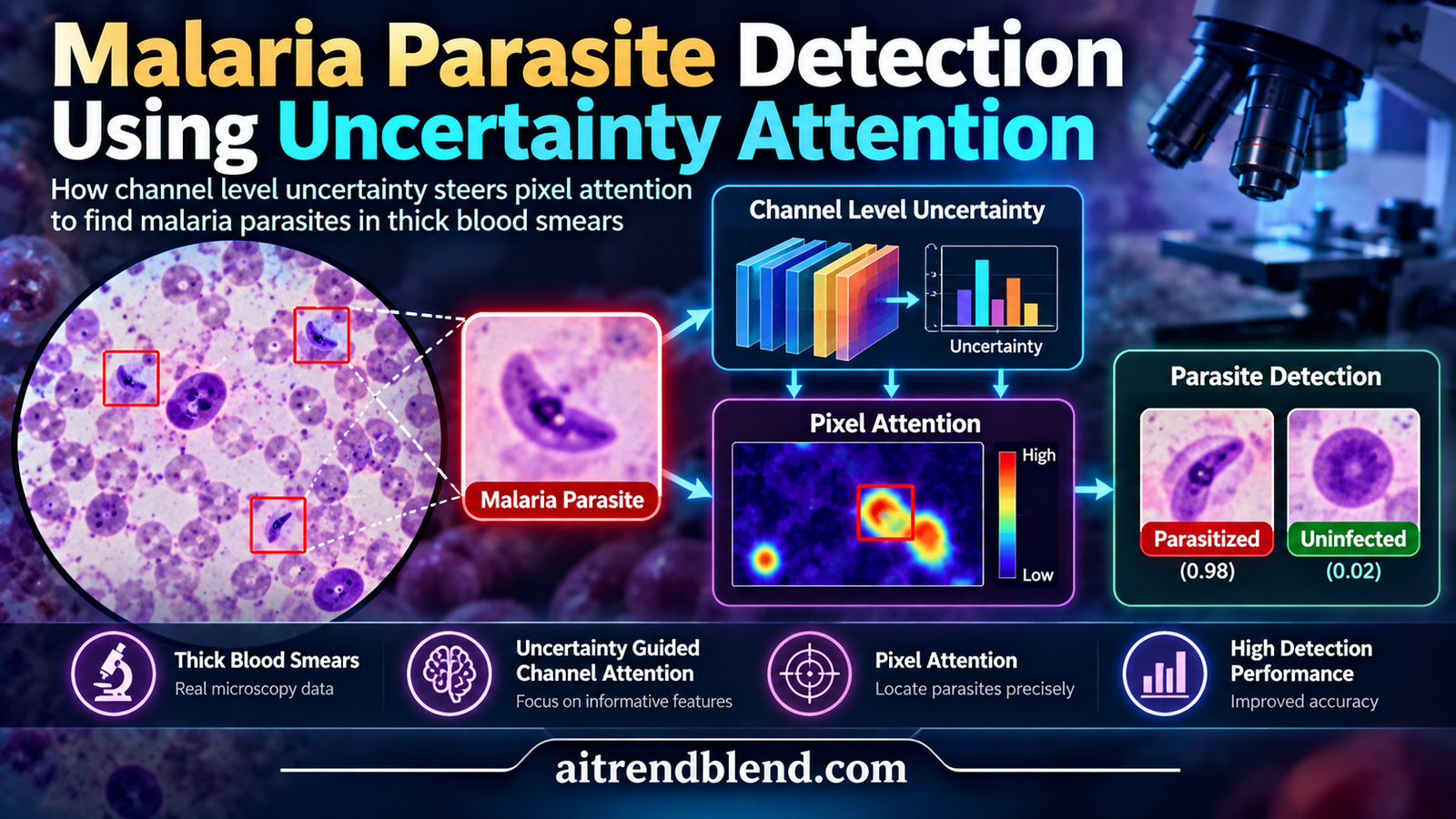
A microscopist leans over a thick blood film under a 100 times objective. The field is a wash of pale purple, and scattered through it are dozens of small dark discs. Some are Plasmodium parasites. Others are stain debris, platelets, or artifacts that soaked up the dye and now look uncomfortably similar. She has to count the real ones, slide after slide, and that count helps decide how sick a patient is judged to be and how fast treatment starts. In the malaria endemic clinics where this work matters most, trained eyes are scarce and tired ones make mistakes.
A 2025 paper in Neural Networks from Macquarie University and the University of Sydney asks a sharper question than most screening research. Not only which specks are parasites, but which parts of the model’s own evidence deserve to be trusted.
Key points
- The method scores each of 64 feature channels for uncertainty, then lets those scores decide how much every channel may contribute to a pixel attention module.
- On the CMM dataset with 13 patients it reaches a parasite level F1 of 59.96 and an AP of 40.73. On Thick Smears 150 with 150 patients it reaches 84.13 and 77.77.
- Our reading of the ablation is that most of the gain over the PDNet baseline on CMM comes from pixel attention, while the uncertainty step adds a smaller and less uniform increment.
- Cost stays close to the baseline at about 1.0 million parameters and roughly 0.82 and 2.15 seconds per image on the two datasets.
- Clinical readiness is not shown. The two datasets were evaluated separately, no slide level diagnosis is reported, and no comparison with human readers appears in the paper.
Why a thick smear is so hard to read
Malaria is passed to people through the bite of an infected mosquito. The World Health Organization report cited by the authors counts 247 million cases and 619,000 deaths worldwide in 2022. The disease is curable, but only when it is recognized in time, and the reference method for recognizing it is still a human being looking through a microscope at stained blood.
Two kinds of film get used. A thin smear spreads blood into a single layer, so red cells are large, flat, and easy to see, and a parasite inside one is a clear target. A thick smear stacks blood in a dense drop that is dried and stained with a Romanowsky type stain. It holds much more blood per field, and the paper puts its sensitivity for low parasite density cases at about eleven times that of a thin film, citing Warhurst and Williams from 1996. That is why thick films are used for counting parasites and gauging severity.
The price of that sensitivity is legibility. In a thick film there are no tidy red cells to anchor the eye. Parasites show up as small, round, purple discs, and other things absorb the stain just as eagerly. White blood cells look similar in color though much larger. The authors call these lookalikes distractors, and they are the reason a naive darkness threshold fails.
Why tiny objects defeat general purpose detectors
Scale makes it worse. The images in this study are large, 2560 by 2160 pixels for CMM and 3024 by 4032 for Thick Smears 150, while a parasite is only around 44 pixels across. A 44 by 44 patch covers roughly 0.016 percent of a 3024 by 4032 frame, which is our own arithmetic from the paper’s numbers.
Now consider what happens to a detector that resizes the whole frame. The paper’s cost table describes the YOLO family models as running on standard 640 by 640 inputs. Squeezing a 3024 by 4032 photograph into that square shrinks a 44 pixel parasite to somewhere between seven and nine pixels. Most of what makes it recognizable is gone before the network sees it. This is the paper’s stated reason for preferring a candidate first approach, and the arithmetic makes the argument feel less like a preference and more like a necessity.
What earlier systems did, and where they stalled
The oldest approaches were hand built. Hanif and colleagues thresholded dark regions after a dark stretching step. Kaewkamnerd and colleagues moved to the HSV color space and worked on the brightness channel with an adaptive threshold. Others computed shape and color features and passed them to a support vector machine or a clustering routine. The authors summarize the verdict plainly. These low level techniques struggle to hold accuracy once stain, focus, and lighting vary.
Deep learning then arrived in two flavors. One family treats parasite finding as object detection, with YOLO variants and relation modules for the class imbalance between infected and healthy cells. Some of these target thin smears. Sukumarran and colleagues, for example, tuned a YOLO model for infected cells in thin films. The other family first proposes candidate patches and then classifies each one. Manescu and colleagues trained a weakly supervised model that only needed each film labeled positive or negative, which eases annotation but, as the authors of this paper point out, gave weaker performance than fully supervised training. Yang and colleagues built PDNet, a compact VGG style classifier on candidate patches that could run on a smartphone. PDNet is the backbone that the present work builds on and the baseline it must beat.
If you follow medical imaging more broadly, you will notice the same tension in other subfields. Our hub on AI for medical imaging and healthcare tracks how these choices between detection and patch classification play out elsewhere.
The gap the authors go after
Uncertainty is not new to medical imaging. Leibig and colleagues used dropout based Bayesian estimates to flag uncertain diabetic retinopathy diagnoses. Kohl and colleagues built a probabilistic U-Net that produces many plausible segmentations. Herzog and colleagues did something similar for stroke lesions on MRI. Nearly all of this work attaches uncertainty to the output, telling you how much to trust the final answer.
The authors argue that nobody in malaria detection has estimated the uncertainty of the learned features themselves and then used it to downweight the shaky ones. That is a narrower and more testable claim than it first sounds, and the rest of the paper is an attempt to show it pays off.
The core idea in plain language
Picture the last convolutional layer as a panel of 64 reviewers. Each looks at the same small patch, forms a view, and hands over a summary in the shape of a 5 by 5 map. A standard channel attention module decides how loudly each reviewer should speak. It gives every channel one number between 0 and 1.
What it does not tell you is how sure each reviewer is on this particular patch. A smudge, an out of focus region, or a piece of debris could confuse some reviewers and leave others untouched. The proposal is to estimate a variance for each channel, treat it as a measure of unreliability, and turn it into a soft weight that shrinks the confused reviewers before anything else happens.
After that comes the second step. Pixel attention asks a different question, which is which positions in the 5 by 5 map matter, and it asks it only over the channels that survived the reliability filter. The paper’s own framing is that its attention hunts for input level reliable features, not for long range relationships the way transformer style attention does.
From slide to verdict, the full pipeline
Before any attention happens, the pipeline shrinks the search space. Following Yang and colleagues, it converts the image to grayscale and applies Otsu’s method to find the white blood cell mask, which is then removed. Parasites are darker than most of the background, so the remaining pixel with the lowest intensity becomes a candidate. A circular region of radius 22 around it is cropped, with everything outside the circle painted black, and the process repeats. This iterative global minimum screening produces 500 patches of 44 by 44 by 3 per image on Thick Smears 150, and 300 per image on CMM.
In total that gives 71,700 candidate patches for CMM and 909,500 for Thick Smears 150. The authors report that 94.52 percent of true parasites in CMM and 97.29 percent in Thick Smears 150 end up inside some candidate patch. Those percentages are a ceiling. Whatever the classifier does next, it cannot recover a parasite that the screening step never proposed.
Each candidate is then classified independently as parasite or distractor, and that independence has a practical consequence. Total compute grows linearly with the number of patches, which is why the same network costs 6.2 GFLOPs on CMM and 10.5 on Thick Smears 150.
Inside the network
The backbone
The feature extractor comes from PDNet and follows a VGG pattern of small 3 by 3 convolutions with batch normalization and ReLU, interleaved with max pooling. Following the widths in the paper’s Figure 3, a 44 by 44 by 3 patch becomes 22 by 22 by 16, then 11 by 11 by 32, then 5 by 5 by 64. The text says the output of the seventh convolutional layer, a 5 by 5 by 64 map, is what feeds the fully connected layers. The classifier has widths of 512 and 50 with dropout at 0.5 and ends in a two way softmax.
Stage one, Bayesian channel attention
In stage one the authors insert a Bayesian channel attention module after that last feature map. Global average pooling squeezes each channel to a single number. Two small branches of 1 by 1 convolutions then predict a mean and a variance for an attention score per channel. A sample is drawn using the reparameterization trick, passed through a sigmoid, and multiplied back onto the features with a residual connection.
The essential point is that the variance depends on the input. A noisy patch can produce high variance in different channels than a clean one, and Figure 5 in the paper shows exactly that, with reliability weights that differ from patch to patch.
Stage two, uncertainty guided pixel attention
Stage two swaps the Bayesian module for pixel attention. Each channel’s variance is converted to a reliability weight, the feature map is scaled by those weights, and a pixel attention branch produces one weight for each of the 25 spatial positions. The result is added back onto the scaled features. Only this second network is described as being used at inference.
Two stage training
Both networks are trained with stochastic gradient descent at a learning rate of 0.0005 and momentum 0.9, for 200 epochs on each dataset. Batches hold 2000 patches. Training used PyTorch 1.7.1 on a single Tesla T4. Evaluation uses five fold cross validation split by patient, so patches from one patient never sit in both training and test sets, and half a percent of the training data is held out for picking the best checkpoint.
The mathematics behind it
The formulation is compact, so it is worth seeing it whole. Start with what standard channel attention does. Global pooling reduces the feature map to one value per channel.
Two convolutions and a sigmoid turn that vector into weights, and the output adds a weighted copy of the input to itself.
The Bayesian version replaces the single score with a random variable. The attention score z follows a Gaussian whose mean and variance both depend on the input x and the network weights, and the weights themselves carry a zero mean isotropic Gaussian prior with precision tau.
Training maximizes the log likelihood of the labels, which involves integrating over both the scores and the weights. That integral cannot be computed directly for a nonlinear network, so the authors follow Gal and Ghahramani and optimize an evidence lower bound instead.
The first divergence vanishes because the two distributions are set to be the same, and the second becomes an L2 penalty. The remaining expectation is estimated by Monte Carlo. Dropout masks supply samples of the weights, and the reparameterization trick supplies samples of the score.
The last expression is a cross entropy plus weight decay, so training looks like ordinary network training with a stochastic attention layer. Then comes the step that matters most. The estimated variance becomes a reliability weight, with a single hyperparameter beta controlling how harshly uncertainty is punished.
Some illustrative arithmetic helps here, and it is ours rather than the paper’s. With beta at 10, a channel with variance 0.05 keeps a weight of about 0.61, while a channel with variance 0.3 is pushed down to about 0.05, close to silence. The paper notes the two limits too. At beta equal to 0 every weight is 1 and the method reduces to ordinary pixel attention. As beta grows without bound, every weight heads to 0 and nothing gets through.
The experimental setting
Two public datasets from different hospitals were used, and they differ in equipment, sample preparation, and staining, which is what the authors offer as evidence of robustness.
| Item | CMM | Thick Smears 150 |
|---|---|---|
| Subjects | 13 | 150 |
| Images | 239 | 1,819 |
| Annotated parasites | 2,986 | 84,961 |
| Image resolution | 2560 by 2160 | 3024 by 4032 |
| Average parasite size | 42 by 44 pixels | radius of 22 pixels |
CMM comes from the University College Hospital in Ibadan, Nigeria, with thick films of 13 patients stained with Giemsa and parasites marked by local microscopists. Thick Smears 150 comes from Chittagong Medical College Hospital in Bangladesh, where slides from 150 patients were photographed through a smartphone camera and an expert reader from the Mahidol Oxford Tropical Medicine Research Unit in Bangkok annotated the parasites.
The gap in size between the two is huge. CMM offers 2,986 parasites and Thick Smears 150 offers 84,961, roughly 28 times more. That difference explains more of the results than any architectural choice, as we will see.
The results, with the numbers in front of us
The authors compare against six baselines across three families. PDNet is the patch classifier. YOLOv5, a tuned YOLOv5 called Yolov5opt, and a modified YOLOv4 are detectors. NesT, RegionViT, and TransMIL are transformer classifiers. Parasite level results pool every parasite in a dataset.
| Method and dataset | Precision | Recall | F1 | AP |
|---|---|---|---|---|
| CMM, YOLOv5 | 49.07 | 63.44 | 55.34 | 37.48 |
| CMM, Yolov5opt | 29.67 | 68.59 | 41.42 | 23.52 |
| CMM, modified YOLOv4 | 45.72 | 48.36 | 47.00 | 25.86 |
| CMM, PDNet | 46.18 | 67.85 | 54.96 | 30.31 |
| CMM, NesT | 41.03 | 21.70 | 28.39 | 16.56 |
| CMM, RegionViT | 43.44 | 22.18 | 29.36 | 14.72 |
| CMM, TransMIL | 32.30 | 22.92 | 26.81 | 11.94 |
| CMM, this method | 51.39 | 71.96 | 59.96 | 40.73 |
| Thick Smears 150, YOLOv5 | 78.99 | 83.52 | 81.19 | 73.83 |
| Thick Smears 150, Yolov5opt | 75.84 | 67.41 | 71.38 | 51.67 |
| Thick Smears 150, modified YOLOv4 | 77.99 | 81.27 | 79.60 | 72.22 |
| Thick Smears 150, PDNet | 82.19 | 82.74 | 82.46 | 76.63 |
| Thick Smears 150, NesT | 76.82 | 80.27 | 78.51 | 75.99 |
| Thick Smears 150, RegionViT | 78.31 | 81.40 | 79.82 | 75.92 |
| Thick Smears 150, TransMIL | 80.64 | 82.17 | 81.66 | 76.26 |
| Thick Smears 150, this method | 83.15 | 85.13 | 84.13 | 77.77 |
Against PDNet, the gaps look different on the two datasets. On CMM the method gains 5.00 points of F1 and 10.42 points of AP. On Thick Smears 150 the gains shrink to 1.67 points of F1 and 1.14 points of AP. Precision on Thick Smears 150 rises by less than one point, from 82.19 to 83.15, and recall by 2.39 points.
The absolute level on CMM deserves a pause. A precision of 51.39 means roughly half of the parasites the system reports are false alarms. A reader could reasonably call that a research prototype rather than a screening tool.
Patient level results and the size of the error bars
The paper also averages metrics across patients and reports a standard deviation. On CMM, this method scores 35.22 precision, 56.62 recall, 37.40 F1, and 36.39 AP, against PDNet at 29.88, 58.34, 34.21, and 33.04. PDNet’s recall is actually higher, which the authors acknowledge. On Thick Smears 150 the method posts 69.35, 81.58, 72.31, and 69.65 against PDNet’s 69.21, 79.51, 70.91, and 67.82.
Now compare those margins with the spread. The patient level standard deviations for this method on Thick Smears 150 run between 14.34 and 23.73 points, while the largest gap over PDNet is 2.07 points. The averages point the right way, yet the patient to patient variation is many times larger than the improvement. The paper reports no significance test, so we cannot say how much of that margin is signal.
Why detectors and transformers lag
Classification based methods beat detection based ones, and the authors give two reasons. The parasites are tiny in huge images, and the patch pipeline hands the classifier vastly more training examples than a detector gets from whole images. The transformers do poorly too, especially on CMM, where NesT, RegionViT, and TransMIL land between 26.81 and 29.36 F1. The authors attribute this to overfitting, since large parameter counts meet small data and 44 by 44 inputs. That explanation is plausible, though it was not tested with pretraining or regularization changes, so treat it as a hypothesis.
One fairness note. Yolov5opt was tuned by its original authors for infected cells in thin smears, so its weak showing on thick films is partly a mismatch of purpose and not a clean verdict on the family.
Compute and speed
| Method | Params (M) | FLOPs CMM (G) | FLOPs Thick (G) | Seconds CMM | Seconds Thick |
|---|---|---|---|---|---|
| YOLOv5 | 9.1 | 12.1 | 12.1 | 0.007 | 0.007 |
| PDNet | 0.9 | 6.2 | 10.4 | 0.818 | 2.148 |
| RegionViT | 12.5 | 36.6 | 61.1 | 0.819 | 2.171 |
| This method | 1.0 | 6.2 | 10.5 | 0.821 | 2.146 |
The attention modules are almost free. Parameters rise from 0.9 to 1.0 million, and the FLOPs and timings are nearly identical to PDNet. Detectors are far faster per image, at 0.007 seconds for YOLOv5, but the classifier timings include candidate preselection, which is where the time goes. For a screening task that is not real time, a couple of seconds per image is unlikely to be the obstacle.
The method improves parasite level F1 and AP on both datasets, and it does so at almost no extra cost. The size of the gain depends heavily on the dataset, large on the small CMM set and modest on Thick Smears 150.
What the ablation really shows
The paper’s ablation compares five attention styles inside the same backbone. Reading it against the PDNet row from the main table tells a more nuanced story than the text does.
| Variant | CMM F1 | CMM AP | Thick F1 | Thick AP |
|---|---|---|---|---|
| PDNet, no attention | 54.96 | 30.31 | 82.46 | 76.63 |
| Self attention | 53.43 | 28.74 | 81.31 | 76.51 |
| Bayesian channel attention | 55.96 | 35.87 | 83.10 | 76.56 |
| Channel attention | 57.42 | 33.34 | 83.20 | 76.28 |
| Pixel attention | 59.60 | 39.98 | 83.26 | 76.49 |
| Multi head, 1 head | 56.53 | 36.07 | 82.95 | 76.65 |
| Multi head, 2 heads | 52.27 | 33.13 | 81.43 | 74.89 |
| Multi head, 4 heads | 47.88 | 28.40 | 80.88 | 74.96 |
| Uncertainty guided pixel attention | 59.96 | 40.73 | 84.13 | 77.77 |
Start with CMM. Plain pixel attention lifts F1 from 54.96 to 59.60, a jump of 4.64 points. Adding the uncertainty weighting on top brings it to 59.96, an extra 0.36. In AP the same step adds 0.75. On that dataset, then, pixel attention does most of the work, and the uncertainty contribution is small enough that we would want repeated runs before calling it real.
The picture changes on Thick Smears 150. There, pixel attention alone moves F1 from 82.46 to 83.26 and actually leaves AP a hair below the baseline at 76.49. The uncertainty step then adds 0.87 points of F1 and 1.28 points of AP, so the extra term accounts for the AP gain outright. This is the strongest evidence in the paper that the uncertainty idea does something, and it comes from the larger and less noisy dataset.
Two more patterns stand out. Bayesian channel attention on its own does not beat ordinary channel attention on F1 in either dataset, though it does on AP. So the estimated variance is not automatically a better channel signal, and its value seems to show up when it gates a second module. Second, adding attention heads makes things steadily worse, from 56.53 F1 with one head down to 47.88 with four on CMM. That fits the overfitting story the authors tell about small data.
The candidate level ROC curves tell a similar tale. On CMM the AUC for the full method is 0.7862, against 0.7824 for pixel attention and 0.7530 for channel attention. On Thick Smears 150 the values are 0.9827 and 0.9781. The differences at the top are small, and a candidate level AUC below 0.79 on CMM shows how hard that dataset remains.
The channel features with higher variance are considered less reliable.Xiong et al., Neural Networks 191 (2025), Introduction
How sensitive is it to beta and patch size?
| Beta | CMM F1 | CMM AP | Thick F1 | Thick AP |
|---|---|---|---|---|
| 1 | 59.82 | 39.80 | 83.09 | 76.59 |
| 10 | 59.96 | 40.73 | 84.13 | 77.77 |
| 20 | 59.87 | 40.56 | 82.51 | 77.03 |
| 100 | 57.98 | 37.40 | 81.22 | 68.20 |
The pattern is an inverted U. At beta equal to 1 most reliability weights sit above 0.85, so almost nothing is filtered and the result is close to plain pixel attention. At 100 many weights fall below 0.5, and information stops flowing, which is why AP on Thick Smears 150 collapses from 77.77 to 68.20, a drop of 9.57 points.
The authors are frank that they did not search exhaustively because training is expensive. They tried four values only. The optimum could sit anywhere between 1 and 20, and it may well differ across datasets. Anyone reproducing the work should treat beta as a parameter to tune and not as a settled constant.
Patch size was also checked at 36, 44, 52, and 60 pixels. The chosen 44 by 44 wins six of nine metrics on CMM and seven on Thick Smears 150. The authors reason that 36 is too small to carry enough context and that 52 and 60 admit more background noise.
A question the paper leaves open
There is one point about the machinery that we could not resolve from the text. The paper states that at inference only the second network is used. Yet Equation 13 needs an input dependent variance, and Figure 3 shows that variance flowing from stage one into stage two. If the stage one network is not run at test time, where does the variance for a new patch come from?
One hint comes from Table 4. The FLOPs for this method equal PDNet’s on CMM at 6.2 giga operations, and parameters differ by only 0.1 million. Running two full backbones would be expected to cost close to double. That suggests the reported cost may count a single backbone, though it does not tell us how the variance is obtained. The authors say data will be made available on request, and code would settle the matter. In our reference implementation below we take the conservative reading and run both networks at inference, which roughly doubles backbone compute.
From benchmark to bedside
Numbers on a benchmark are one thing. A tool that helps a clinician decide is another, and the gap between them deserves plain language.
Clinical translation gap
The paper measures how well individual parasites are localized, using precision, recall, F1, and AP. A working screening service needs more. It must turn detections into a parasite density per unit of blood, decide whether a slide is positive or negative, and ideally identify the species. The authors argue that their approach allows severity estimation and patient prioritization, but no experiment in the paper maps detections to density or to a slide level diagnosis, and no sensitivity or specificity for diagnosis is reported.
The evaluation is also single source on each side. Each dataset is trained and tested on its own, with five folds. The authors emphasize that the two datasets differ in equipment and staining, yet no model trained on one is tested on the other. A smartphone photograph from Bangladesh and a digitized field from Nigeria are different worlds, and real deployment brings a third and fourth. We do not know how the method behaves when a clinic uses a new microscope, a different stain batch, or a different phone.
Ground truth matters too. The 84,961 parasites in Thick Smears 150 were annotated by one expert reader, so inter reader variability, which is well known in microscopy, is unknown here. And no head to head with practicing microscopists is included. That comparison is what clinicians will ask for first.
Regulatory and safety notes
Software that informs diagnosis is generally treated as a medical device in many jurisdictions, and it typically needs validation on the intended population, equipment, and workflow before clinical use. Nothing in this paper claims otherwise, and it should not be read as evidence of clearance.
Two error types carry different risks. A missed parasite, which can happen if the preselection step never proposes it, may delay treatment. A false alarm may lead to unnecessary treatment or extra testing. The authors suggest that patches dominated by unreliable features could be flagged for manual review. That is a sensible safety design, though the paper describes the idea and does not test it. Prefer to think of any such system as decision support with a human reader in the loop.
Where the idea could travel
The conceptual move here is portable. Estimating uncertainty over features and using it to gate later computation could apply anywhere inputs vary in noise, and the authors mention histopathology and dermatology images. That is a suggestion and not a result, since nothing outside malaria was tested. Their Figure 5 also opens an interpretability angle. Reliability weights that change patch by patch could act as a built in signal about how trustworthy a prediction is.
For readers who work on attention more generally, this sits in an interesting corner. Most recent attention research chases global context. This work asks which features to believe, which is a different axis. Our coverage of attention mechanisms in vision models and our related piece on deep learning for other microscopy tasks give useful contrast. Another medical imaging analysis on our site looks at uncertainty from the output side.
Honest limitations
The authors list two limitations themselves. Performance depends on the candidate preselection stage, with ceilings of 94.52 percent on CMM and 97.29 percent on Thick Smears 150, and a parasite missed there cannot be recovered. Training also takes two stages, which complicates a move to a single end to end pipeline.
We would add several more.
Sample size. CMM has 13 patients. With five folds split by patient, each test fold holds only two or three people, so patient level averages rest on very few individuals. The 2,986 parasites and 239 images are also modest for training a network that is then evaluated at the level of a single patient.
Dataset bias. Both datasets come from single institutions with specific stains and, in one case, a specific smartphone setup. Thick Smears 150 has one expert annotator. Geographic, equipment, and annotator effects cannot be separated from the method’s performance.
Generalization. No cross dataset test is reported, and no external site was used. The claim of robustness rests on the fact that two different datasets each gave good numbers, which is weaker than showing transfer.
Statistical evidence. No confidence intervals or significance tests appear, and parasite level scores come without variability across folds. Several improvements, especially the ablation gains on CMM, are smaller than one point.
Reproducibility. The data availability statement says data will be provided on request. There is no public code, and the inference wiring described above is unclear.
Read the paper as a promising and cheap way to make an established patch classifier more robust to noise. Do not read it as proof that automated thick smear diagnosis is ready for the clinic. The missing steps are external validation, slide level diagnosis, and comparison with human readers.
A reference implementation in PyTorch
The listing below is our own independent implementation written from the paper’s description. It is not the authors’ code. Where the paper is silent, such as padding, the bottleneck width of the attention branches, and the exact way the variance is kept positive, we made a choice and marked it in a comment. The backbone follows the layer widths in Figure 3. Treat the listing as a starting point for your own experiments, and run the smoke test at the bottom on your machine before building on it.
"""
Uncertainty guided attention learning for malaria parasite classification.
Independent reference implementation written from the description in
Xiong et al., Neural Networks 191 (2025) 107833.

Stage 1 trains a backbone with Bayesian channel attention and yields a
per channel variance. Stage 2 trains the same backbone with uncertainty
guided pixel attention that consumes exp(-beta * variance).

Layer widths follow Figure 3 of the paper. Where the paper is silent
(padding, the exact variance parameterisation, the bottleneck ratio of the
pixel attention) the choices below are ours and are marked in comments.
"""
import torch
import torch.nn as nn
import torch.nn.functional as F


# ---------------------------------------------------------------------------
# 1. Backbone (feature extraction), derived from the VGG style PDNet layout
# ---------------------------------------------------------------------------
def conv_bn_relu(c_in, c_out):
    return [nn.Conv2d(c_in, c_out, 3, padding=1),
            nn.BatchNorm2d(c_out),
            nn.ReLU(inplace=True)]


class Backbone(nn.Module):
    """Input 3x44x44, output 64x5x5 after the 7th convolution."""

    def __init__(self):
        super().__init__()
        layers = []
        layers += conv_bn_relu(3, 16) + conv_bn_relu(16, 16) + [nn.MaxPool2d(2)]    # 22x22x16
        layers += conv_bn_relu(16, 32) + conv_bn_relu(32, 32) + [nn.MaxPool2d(2)]   # 11x11x32
        layers += conv_bn_relu(32, 64) + conv_bn_relu(64, 64) + [nn.MaxPool2d(2)]   # 5x5x64
        layers += conv_bn_relu(64, 64)                                              # 7th conv
        self.body = nn.Sequential(*layers)

    def forward(self, x):
        return self.body(x)


# ---------------------------------------------------------------------------
# 2. Bayesian channel attention (Equations 1 to 5 and 11)
# ---------------------------------------------------------------------------
class BayesianChannelAttention(nn.Module):
    """
    Global pooling gives g_c. Two 1x1 conv branches predict the mean and the
    variance of the attention score z. A reparameterised sample of z goes
    through a sigmoid, and the output is F + a * F as in Equation 3.
    """

    def __init__(self, channels=64, reduction=4):
        super().__init__()
        hidden = max(channels // reduction, 1)
        self.mu = nn.Sequential(nn.Conv2d(channels, hidden, 1), nn.ReLU(inplace=True),
                                nn.Conv2d(hidden, channels, 1))
        self.var = nn.Sequential(nn.Conv2d(channels, hidden, 1), nn.ReLU(inplace=True),
                                 nn.Conv2d(hidden, channels, 1))

    def forward(self, feat):
        g = feat.mean(dim=(2, 3), keepdim=True)               # Equation 1
        mu = self.mu(g)
        # Our choice, softplus keeps the variance positive and stable.
        sigma2 = F.softplus(self.var(g)) + 1e-6
        eps = torch.randn_like(mu)
        z = mu + torch.sqrt(sigma2) * eps                      # Equation 11
        a = torch.sigmoid(z)                                   # Equation 5
        out = feat + a * feat                                  # Equation 3
        return out, sigma2                                     # sigma2 has shape B x C x 1 x 1


# ---------------------------------------------------------------------------
# 3. Uncertainty guided pixel attention (Equations 13 to 15)
# ---------------------------------------------------------------------------
class UncertaintyGuidedPixelAttention(nn.Module):
    def __init__(self, channels=64, beta=10.0, reduction=8):
        super().__init__()
        self.beta = beta
        hidden = max(channels // reduction, 1)
        # One channel output gives a weight for every pixel, size H x W.
        self.pa = nn.Sequential(nn.Conv2d(channels, hidden, 1), nn.ReLU(inplace=True),
                                nn.Conv2d(hidden, 1, 1), nn.Sigmoid())

    def forward(self, feat, sigma2):
        w_sigma = torch.exp(-self.beta * sigma2)               # Equation 13
        f_tilde = feat * w_sigma                               # reliable features
        a_p = self.pa(f_tilde)                                 # Equation 14
        out = f_tilde + a_p * f_tilde                          # Equation 15
        return out, w_sigma


# ---------------------------------------------------------------------------
# 4. Classification head shared by both stages
# ---------------------------------------------------------------------------
class Head(nn.Module):
    def __init__(self, channels=64, p_drop=0.5):
        super().__init__()
        self.net = nn.Sequential(
            nn.Flatten(),
            nn.Linear(channels * 5 * 5, 512), nn.ReLU(inplace=True), nn.Dropout(p_drop),
            nn.Linear(512, 50), nn.ReLU(inplace=True), nn.Dropout(p_drop),
            nn.Linear(50, 2))

    def forward(self, x):
        return self.net(x)


# ---------------------------------------------------------------------------
# 5. The two networks
# ---------------------------------------------------------------------------
class Stage1Net(nn.Module):
    """Backbone, Bayesian channel attention, classifier. Yields channel variance."""

    def __init__(self):
        super().__init__()
        self.backbone = Backbone()
        self.attn = BayesianChannelAttention(64)
        self.head = Head(64)

    def forward(self, x):
        f = self.backbone(x)
        f, sigma2 = self.attn(f)
        return self.head(f), sigma2


class Stage2Net(nn.Module):
    """Backbone, uncertainty guided pixel attention, classifier."""

    def __init__(self, beta=10.0):
        super().__init__()
        self.backbone = Backbone()
        self.attn = UncertaintyGuidedPixelAttention(64, beta=beta)
        self.head = Head(64)

    def forward(self, x, sigma2):
        f = self.backbone(x)
        f, w_sigma = self.attn(f, sigma2)
        return self.head(f), w_sigma


# ---------------------------------------------------------------------------
# 6. Loss, the practical form of the ELBO in Equation 12
# ---------------------------------------------------------------------------
def elbo_loss(logits, target, model, l2=5e-4):
    """
    Negative log likelihood of the labels plus an L2 penalty on the weights.
    The KL terms in Equation 10 collapse to this L2 term, as the paper explains.
    """
    nll = F.cross_entropy(logits, target)
    reg = sum((p ** 2).sum() for p in model.parameters() if p.requires_grad)
    return nll + l2 * reg


# ---------------------------------------------------------------------------
# 7. Training loops
# ---------------------------------------------------------------------------
def make_optimizer(model, lr=5e-4, momentum=0.9):
    return torch.optim.SGD(model.parameters(), lr=lr, momentum=momentum)


def train_stage1(model, loader, epochs, device="cpu"):
    model.to(device).train()
    opt = make_optimizer(model)
    for ep in range(epochs):
        total = 0.0
        for x, y in loader:
            x, y = x.to(device), y.to(device)
            logits, _ = model(x)
            loss = elbo_loss(logits, y, model)
            opt.zero_grad()
            loss.backward()
            opt.step()
            total += loss.item()
        print(f"stage 1 epoch {ep + 1} loss {total / max(len(loader), 1):.4f}")
    return model


@torch.no_grad()
def channel_variance(stage1, x, samples=1):
    """Average sigma squared over a few stochastic passes of the stage 1 net."""
    stage1.eval()
    acc = 0.0
    for _ in range(samples):
        _, s2 = stage1(x)
        acc = acc + s2
    return acc / samples


def train_stage2(stage2, stage1, loader, epochs, device="cpu"):
    stage1.to(device).eval()
    stage2.to(device).train()
    opt = make_optimizer(stage2)
    for ep in range(epochs):
        total = 0.0
        for x, y in loader:
            x, y = x.to(device), y.to(device)
            s2 = channel_variance(stage1, x)
            logits, _ = stage2(x, s2)
            loss = elbo_loss(logits, y, stage2)
            opt.zero_grad()
            loss.backward()
            opt.step()
            total += loss.item()
        print(f"stage 2 epoch {ep + 1} loss {total / max(len(loader), 1):.4f}")
    return stage2


# ---------------------------------------------------------------------------
# 8. Evaluation, precision, recall, F1 and average precision
# ---------------------------------------------------------------------------
def average_precision(scores, labels):
    """Area under the precision recall curve using the step definition."""
    order = torch.argsort(scores, descending=True)
    labels = labels[order].float()
    tp = torch.cumsum(labels, 0)
    fp = torch.cumsum(1 - labels, 0)
    precision = tp / (tp + fp).clamp(min=1)
    recall = tp / labels.sum().clamp(min=1)
    prev_recall = torch.cat([torch.zeros(1), recall[:-1]])
    return float(((recall - prev_recall) * precision).sum())


@torch.no_grad()
def evaluate(stage2, stage1, loader, device="cpu", threshold=0.5):
    stage1.to(device).eval()
    stage2.to(device).eval()
    all_p, all_y = [], []
    for x, y in loader:
        x = x.to(device)
        s2 = channel_variance(stage1, x)
        logits, _ = stage2(x, s2)
        all_p.append(F.softmax(logits, dim=1)[:, 1].cpu())
        all_y.append(y)
    p, y = torch.cat(all_p), torch.cat(all_y)
    pred = (p >= threshold).long()
    tp = int(((pred == 1) & (y == 1)).sum())
    fp = int(((pred == 1) & (y == 0)).sum())
    fn = int(((pred == 0) & (y == 1)).sum())
    precision = tp / max(tp + fp, 1)
    recall = tp / max(tp + fn, 1)
    f1 = 2 * precision * recall / max(precision + recall, 1e-12)
    return {"precision": precision, "recall": recall, "f1": f1,
            "ap": average_precision(p, y)}


# ---------------------------------------------------------------------------
# 9. Smoke test on dummy data
# ---------------------------------------------------------------------------
if __name__ == "__main__":
    torch.manual_seed(0)
    n = 64
    x = torch.rand(n, 3, 44, 44)
    y = (torch.rand(n) < 0.2).long()
    ds = torch.utils.data.TensorDataset(x, y)
    loader = torch.utils.data.DataLoader(ds, batch_size=16, shuffle=True)

    s1 = Stage1Net()
    s2 = Stage2Net(beta=10.0)
    train_stage1(s1, loader, epochs=2)
    train_stage2(s2, s1, loader, epochs=2)
    print(evaluate(s2, s1, loader))
    logits, w = s2(x[:4], channel_variance(s1, x[:4]))
    print("logits", tuple(logits.shape), "reliability weights", tuple(w.shape))
The training loops follow the two stage recipe, with the second network consuming the variance of the first. The evaluation function reports precision, recall, F1, and average precision on patch labels. To reproduce the paper’s parasite level numbers you would also need the candidate generation step from Yang and colleagues and the patient wise five fold split.
Conclusion
The core achievement is modest in the best sense. The authors took a compact, established classifier and added attention modules that cost about 0.1 million parameters and nearly no extra compute. In return they report better parasite level F1 and average precision on two public datasets, including a 10.42 point gain in AP on CMM and the best AP on both datasets in the parasite and patient level tables.
The conceptual shift is the more interesting part. Most uncertainty work in medical imaging asks how much to trust an answer. This paper asks how much to trust each ingredient before the answer is formed, and lets that trust reshape what the next layer sees. The reliability weight in Equation 13 is a small formula, yet it makes the network’s internal evidence explicit and inspectable.
Whether that idea transfers is an open question. Histopathology, dermatology, and other imaging tasks share the noise problem, and the authors point that way. But the ablation shows that on the smaller dataset most of the gain came from pixel attention, and the uncertainty step delivered its clearest benefit on the larger one. Any group trying the idea elsewhere should run that same decomposition, so they know which part they are buying.
The limits are just as clear. Two small and single source datasets, no external validation, no slide level diagnosis, no test against microscopists, and an inference pipeline that is not fully specified. Those gaps do not undermine the contribution as a method paper, but they decide how far a reader should trust it as a clinical claim.
The next steps are easy to name. Train on one site and test on another. Convert parasite detections into density and slide level calls and compare with expert readers. Report variability and significance. Test the idea of flagging low confidence patches for manual review, which the authors propose. Release code so the inference question can be closed. If those pieces fall into place, uncertainty guided attention could become a useful part of screening in the places that need it most.
A network that knows which of its own features to doubt is a small step toward tools that clinicians can actually trust.
Frequently asked questions
What makes thick blood smears harder to read than thin smears for malaria detection
A thick smear packs more blood into a small area, which raises its sensitivity for low density infections by roughly eleven times compared with a thin smear according to the source the authors cite. That density also destroys the clean red cell outlines a thin smear provides, so parasites appear only as small round purple discs and other stained debris can look almost the same.
What is Bayesian channel attention and how does it differ from ordinary channel attention
Ordinary channel attention assigns each feature channel one importance score. Bayesian channel attention treats that score as a random variable with a mean and a variance, so the network also learns how uncertain each channel’s importance is for a given input patch. Channels with higher variance are treated as less trustworthy.
How does uncertainty guided pixel attention use the estimated variance
The variance from the Bayesian channel attention stage is converted into a reliability weight between zero and one using the formula exp of negative beta times sigma squared. That weight scales each channel before a pixel attention module looks for the most informative spatial positions, so unreliable channels contribute less to the final decision.
How much better is this method than the PDNet baseline it builds on
On the CMM dataset it improves parasite level F1 from 54.96 to 59.96 and average precision from 30.31 to 40.73. On Thick Smears 150 the gains are smaller, F1 rises from 82.46 to 84.13 and average precision from 76.63 to 77.77. The larger dataset shows a steadier but more modest improvement.
Is this system ready to diagnose malaria in a clinic
Not based on what the paper reports. It evaluates parasite level detection accuracy on two research datasets and does not test slide level diagnosis, parasite density estimation, cross site generalization, or comparison against practicing microscopists. Readers should treat it as promising research rather than a validated clinical tool.
What does the hyperparameter beta control and how was it chosen
Beta controls how aggressively the reliability weight punishes uncertain channels. A low beta barely filters anything, and a very high beta blocks almost all information from every channel. The authors tested four values, one, ten, twenty, and one hundred, and found ten gave the best results on both datasets, though they note they did not run an exhaustive search.
Read the source and explore the data. The paper is open access, and the authors say their data can be requested.
Read the full paperFor the primary source, see the open access article in Neural Networks, and for background on where this fits, visit our AI for medical imaging hub.
Xiong, H., Wang, Z., Sharan, R. V., & Berkovsky, S. (2025). Uncertainty-guided attention learning for malaria parasite detection in thick blood smears. Neural Networks, 191, 107833. Published open access under a CC BY license.
This analysis is based on the published paper and an independent evaluation of its claims.