
Key points
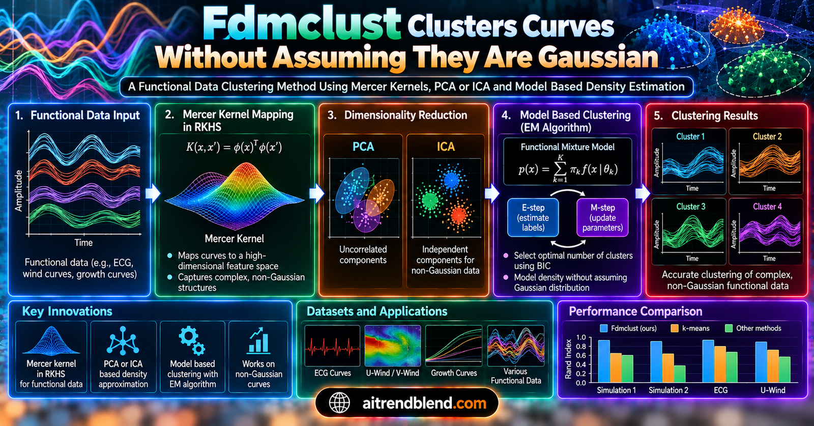
- Fdmclust is a model based clustering method for functional data, meaning entire curves rather than fixed length vectors, that works for both Gaussian and non Gaussian data.
- It projects curves onto a Mercer kernel, a more general and often nonlinear alternative to the covariance kernel used by earlier methods, then proves that the resulting projection coefficients are correlated rather than independent, contrary to what prior work assumed.
- To recover independence, it applies principal component analysis when the data is Gaussian and independent component analysis when it is not, checked automatically with a Shapiro-Wilk test.
- Cluster assignment runs through a finite mixture model fit with the expectation maximization algorithm, using kernel density estimates of the decorrelated components as the per cluster density.
- On ten simulated and real datasets it consistently matches or beats funHDDC and Funclust, the two established model based competitors, and on two the improvement is large, seventy nine and a half percent on a noisy signal dataset and forty two percent on a signal shape dataset, both measured by Rand Index.
- On real wind data from Alberta the clusters it finds line up with the province’s actual north to south geography noticeably better than Funclust’s clusters do.
Why clustering a curve is not like clustering a point
Ordinary clustering algorithms expect a table of numbers, one row per observation, a fixed number of columns. Functional data breaks that format on purpose. A growth curve, a wind speed trace, a spectrometric absorbance reading, each one is a continuous function, observed at some number of time points that may not even be the same across observations. The field built around this kind of data, functional data analysis, has its own toolkit, and one recurring move in that toolkit is projecting each curve onto a basis of functions so that clustering can happen in coefficient space rather than curve space.
The question this paper by Hanieh Saeidi, Mina Aminghafari, and Mehdi Ashkartizabi picks up is what happens to those coefficients once the projection is not the simplest possible choice. Specifically, when you project a curve onto the eigenfunctions of a Mercer kernel, a general symmetric positive definite kernel that includes the ordinary covariance kernel as one special case, do the resulting coefficients behave the way a widely used prior method assumed they would.
The assumption that turns out not to hold
To define a probability density for a random function at all, you need some notion of independence among the coefficients that describe it, since a function technically lives in an infinite dimensional space where the usual density machinery does not directly apply. Delaigle and Hall worked out a way to approximate that density using the small ball probability of a function, projected onto the eigenfunctions of its own covariance kernel. When the underlying data is Gaussian, projecting onto the covariance kernel produces coefficients that are not just uncorrelated but genuinely independent, which is exactly the property their approximation needs, and it was on this foundation that Jacques and Preda built Funclust, one of the two established model based clustering methods this paper compares against.
The Mercer kernel is attractive precisely because it does not require the strict Gaussian assumption and can capture nonlinear structure the covariance kernel misses. But that flexibility comes at a cost the paper works out explicitly. Projecting a function onto the eigenfunctions of a Mercer kernel instead of the covariance kernel produces coefficients whose covariance is a weighted sum involving the original covariance kernel’s eigenvalues and the overlap between the two sets of eigenfunctions.
That sum is, in the paper’s own words, generally nonzero, which means the coefficients are not uncorrelated, let alone independent. This is not a minor technical footnote. It means anyone who projects functional data onto a Mercer kernel and then plugs the result directly into a density approximation built on the independence assumption is working from a foundation that quietly does not hold.
Two different fixes for two different kinds of data
Once the paper establishes that Mercer kernel coefficients are correlated, it needs some other route back to independence, since independence is still what the density approximation requires. It splits into two cases depending on whether the underlying functional data is Gaussian or not, and this split is the practical heart of the method.
If the data is Gaussian, ordinary principal component analysis is enough. For Gaussian data, uncorrelated is equivalent to independent, so decorrelating the projection coefficients with PCA recovers exactly the property the density approximation needs. If the data is not Gaussian, PCA only guarantees the weaker property of zero correlation, which is not sufficient, so the paper turns to independent component analysis instead, a technique built specifically to separate a set of mixed signals into components that are statistically independent rather than merely uncorrelated. Whether to take the Gaussian or the non Gaussian branch is decided automatically with a Shapiro-Wilk normality test on the projected coefficients.
What the density approximation actually looks like once you have independence back
With independent components in hand, the paper proves a small ball probability theorem that plays the same role Delaigle and Hall’s original result played, but for the Mercer kernel case. The resulting density approximation is a simple product across the independent components.
Here each \( d_j \) is the one dimensional density of the jth independent or principal component, estimated in practice with an ordinary kernel density estimator, and q is a truncation point chosen so that only the components carrying meaningful signal are kept, decided in the paper using Cattell’s scree test with a threshold of point zero five. This product form is what makes the whole approach tractable. Instead of trying to estimate a density directly on an infinite dimensional space of functions, which is not really possible, the method reduces the problem to estimating q separate one dimensional densities and multiplying them together.
Turning a density approximation into an actual clustering algorithm
A density approximation alone does not cluster anything. To get from there to Fdmclust, the paper wraps the per curve density in a finite mixture model, one component per cluster, each with its own set of variance or scale parameters for the decorrelated coefficients.
Fitting this mixture uses the expectation maximization algorithm, alternating between computing the probability that each curve belongs to each cluster given the current parameter estimates, and updating the parameters given those probabilities.
The paper works out closed form updates for two specific choices of component density, Gaussian and Laplace, which cover the case where the decorrelated coefficients look approximately normal and the heavier tailed case where they do not. EM is initialized using an ordinary K-means run on the raw curves, capped at two hundred iterations.
The five step recipe, stated plainly
Stripped of the notation, the Fdmclust algorithm runs in five steps. Project every curve onto the eigenfunctions of a chosen Mercer kernel to get the raw coefficients. Test whether those coefficients look Gaussian, and if not, run independent component analysis instead of principal component analysis to decorrelate them. Approximate the density of each curve as a product of one dimensional densities of the decorrelated components. Build the pseudo complete log likelihood for a finite mixture over these densities. Run EM to estimate the mixture weights, the per cluster scale parameters, and the cluster assignments.
What actually happened when they tested it
The evaluation is broad by the standards of a methods paper, four simulated datasets with known ground truth clusters and six real datasets, three with known clusters, three without. For the labeled datasets, performance is measured with the Rand Index, which scores how well the predicted partition of curves agrees with the true one, running from zero to one. For the datasets with no known ground truth, the paper falls back to mean square distance from each cluster’s own center, where lower is better, plus a geography based sanity check for the two wind datasets.
| Dataset | Metric | funHDDC | Funclust | Best Fdmclust (kernel and projection) |
|---|---|---|---|---|
| Waves | Rand Index | 0.99 | 0.77 | 1.00 (PCA, any kernel) |
| Irrationals | Rand Index | 0.54 | 0.55 | 0.55 (PCA, tie with Funclust) |
| Group 1 | Rand Index | not computed | 0.60 | 0.85 (PCA, wavelet kernel) |
| Signals | Rand Index | not computed | 0.49 | 0.88 (PCA, Gaussian kernel) |
| Spectrometric | Rand Index | 0.60 | 0.56 | 0.64 (ICA, Laplacian kernel) |
| ECG | Rand Index | 0.56 | 0.57 | 0.64 (PCA, any kernel) |
| Growth | Rand Index | 0.50 | 0.57 | 0.70 (ICA, Gaussian kernel) |
| Canadian temperature | MSD, lower is better | 298.50 | 310.06 | 297.06 (PCA, any kernel) |
| Radar | MSD, lower is better | 344.08 | 382.27 | 331.09 (PCA, any kernel) |
| U-Wind | MSD, lower is better | 48.14 | 47.34 | 46.97 (ICA, Laplacian kernel) |
| V-Wind | MSD, lower is better | not computed | 36.63 | 36.32 (ICA, wavelet kernel) |
Two things stand out in that table beyond the fact that Fdmclust wins or ties on every single row. The size of the win varies a great deal by dataset. On the Signals dataset, where curves share a trend but differ in the type of noise corrupting them, the best Fdmclust configuration reaches a Rand Index of 0.88 against Funclust’s 0.49, a seventy nine and a half percent improvement the paper reports directly. On the Irrationals dataset, the improvement essentially disappears, the two methods tie at 0.55. That is a more honest picture than a method that claims uniform dominance, and it is worth noticing which kind of dataset produces the big wins. Signals and Group 1, the two datasets with the largest gains, are both explicitly constructed with heavier tailed or non standard noise, exactly the regime where the Gaussian assumption behind Funclust should be expected to strain.
The second thing worth noticing is which projection wins where. PCA based Fdmclust dominates the simulated datasets and several of the real ones, while ICA based Fdmclust wins specifically on the two real world climate datasets, U-Wind and V-Wind. That split is not an accident. The paper’s own boxplots show the ICA variants carry more run to run variability than the PCA variants across the board, so ICA is winning on the wind data despite being the noisier estimator on average, which suggests the wind data genuinely departs from Gaussian behavior in a way the ICA machinery is built to handle and PCA is not.
The proposed method is applicable to both Gaussian and non Gaussian functional data Saeidi, Aminghafari, and Ashkartizabi, Neurocomputing, 2025
A sanity check that does not depend on any statistic at all
The most convincing piece of evidence in the paper is arguably not in the results table. For the Alberta wind speed data, the true clusters are unknown, so the authors plotted where the clustered weather stations actually sit on a map. Fdmclust groups northern stations, High Level, Fort Vermilion, Peace River, and Grande Prairie, into one cluster and the southern and southeastern stations into another, a division that lines up with how wind behavior is known to vary by latitude in that region. Funclust, run on the same data, misclassifies High River, a station that sits geographically close to the other southern stations but that Funclust places with the northern group.
What the Gaussian versus non Gaussian split actually buys you
It is worth being precise about what problem this solves, because it is easy to overstate. Fdmclust does not claim to always outperform every alternative by a wide margin, the Irrationals dataset shows it can tie. What it claims, and what the correlation proof backs up mathematically, is that the previous generation of density based functional clustering methods rested on an independence assumption that only strictly holds for Gaussian data projected onto its own covariance kernel. The moment you want the extra flexibility of a general Mercer kernel, whether because your data has heavier tails, nonlinear structure, or you simply want a kernel choice that is not tied to the data’s own covariance, that independence assumption silently breaks, and Fdmclust is the fix that lets you keep the flexibility without keeping the broken assumption.
Where the paper is candid about its limits
The authors do not present this as a method that wins everywhere, and it is worth restating the honest parts plainly.
- On the Irrationals dataset, the improvement over funHDDC is described in the paper itself as only a slight one, around one point eight five percent, and Fdmclust ties rather than beats Funclust there.
- The ICA based variants of Fdmclust show noticeably more run to run variability than the PCA based variants across the boxplots reported for every dataset, and generally lower median performance, which means the choice between PCA and ICA is not free of cost even when ICA is the theoretically correct choice for non Gaussian data.
- Kernel parameters are tuned per dataset by a grid search minimizing reconstruction error, reported in a table with a different parameter value for nearly every dataset, which means applying this method to a new dataset is not a plug and play exercise, it requires its own tuning pass.
- For the two real world datasets with no known ground truth, Canadian temperature and Radar, the number of clusters was fixed to match what prior papers had chosen rather than derived independently for this study, and for the ERA5 wind datasets the number of clusters was chosen using the Bayesian Information Criterion, which is a standard but still model dependent choice rather than a discovered fact about the data.
A reference implementation of the core mechanism
The paper’s own implementation lives in R, built on packages including fda, Funclustering, and funHDDC. The block below is an independent Python implementation of the core mechanism it describes, written to make the moving pieces concrete rather than to reproduce the authors’ own code. It covers building a Gaussian Mercer kernel matrix, projecting sampled curves onto its empirical eigenfunctions, testing Gaussianity with a Shapiro-Wilk test, decorrelating with PCA or ICA depending on the result, estimating one dimensional densities with kernel density estimation, and running a simplified EM loop to assign cluster labels.
Two caveats worth stating plainly. This smoke test refits a full kernel density estimate for each cluster on every EM iteration for clarity, which is far slower than a real implementation would need to be, and it uses a fixed Gaussian kernel bandwidth choice rather than the grid search over kernel parameters the paper performs per dataset. Both are simplifications made for readability, not the choices a production implementation should keep.
Why this matters beyond curve clustering specifically
The broader lesson here generalizes past functional data. Whenever a method’s validity rests on an independence assumption that was only ever proven for one specific case, generalizing the method by swapping in a more flexible component, here a Mercer kernel in place of a covariance kernel, can silently break the thing that made the original approach mathematically sound in the first place. The response worth remembering is not to avoid the more flexible component, since the Mercer kernel genuinely does capture nonlinear structure the covariance kernel cannot. The response is to check what the flexible version actually implies for the assumption you are relying on, which is exactly what the correlation proof in this paper does, and to build a specific, matched fix, PCA for the case where the original assumption still nearly holds and ICA for the case where it does not.
Conclusion
Fdmclust’s real contribution is narrower and more precise than a leaderboard entry. It identifies a specific, previously unstated gap between what a general Mercer kernel projection actually produces and what the Delaigle and Hall density approximation, and the Funclust method built on it, assumed that projection would produce. The gap is a lack of independence among the projection coefficients, proven directly rather than asserted, and the fix is a branching strategy, PCA when the underlying functional data is Gaussian and ICA when it is not, decided automatically with a normality test rather than left to the user’s judgment.
The results back up that this is more than a theoretical patch. Across ten datasets Fdmclust matches or beats the two established model based competitors, funHDDC and Funclust, with the largest gains concentrated exactly where you would expect them, datasets built with heavier tailed or structurally non Gaussian noise. The geographic sanity check on the Alberta wind data is arguably the most convincing single piece of evidence in the paper, since it does not depend on any metric at all, just on whether the resulting clusters correspond to something physically real.
Where this could go next follows from the paper’s own honest accounting of where it is weakest. The ICA based variants carry more variance than the PCA based ones, so a more stable way to estimate independent components for functional data would likely improve the method’s worst case behavior. The per dataset kernel parameter tuning is also a real practical cost, and a way to choose or adapt the kernel automatically, rather than through a grid search repeated for every new dataset, would make the method considerably easier to deploy outside a research setting.
The honest limitations are worth naming directly rather than skating past. A tie rather than a win on the Irrationals dataset, a small one point eight five percent gain over funHDDC specifically, noticeably higher run to run variability for the ICA variants across every dataset tested, and a cluster count for two of the three unlabeled real datasets that was carried over from prior papers rather than independently derived. None of that undercuts the core proof, it just marks the edges of what has actually been demonstrated.
What is worth carrying away from this paper is not the Rand Index numbers. It is the correlation calculation itself, a reminder that swapping in a more general tool for a specific one is never automatically safe, and that the honest response is to work out exactly what breaks and fix that, rather than assuming the more general tool inherits the older one’s guarantees for free.
Frequently asked questions
What problem does Fdmclust actually solve
It provides a way to define and estimate a probability density for functional data, meaning entire curves rather than fixed length vectors, that works whether the underlying data is Gaussian or not, and then uses that density inside a mixture model to cluster the curves.
Why does using a Mercer kernel instead of a covariance kernel matter
A covariance kernel only captures linear dependencies in the data and is tied to the data’s own variance structure, while a Mercer kernel is more general and can capture nonlinear correlations, but the paper proves that projecting onto a Mercer kernel produces coefficients that are correlated rather than independent, which breaks the assumption earlier density based methods relied on.
How does the method decide whether to use PCA or ICA
It runs a Shapiro-Wilk normality test on the projected coefficients. If the data looks Gaussian, principal component analysis is enough to recover independence, since uncorrelated and independent are equivalent for Gaussian variables. If the data does not look Gaussian, the method switches to independent component analysis instead.
How well does Fdmclust actually perform compared to existing methods
Across ten simulated and real datasets it matches or beats funHDDC and Funclust on every one measured by Rand Index or mean square distance, with especially large gains on datasets built with non standard or heavy tailed noise, though the margin is small or a tie on at least one dataset, Irrationals, where the paper is direct about that result.
Does this method use deep learning
No. It is a classical statistical method built on kernel eigendecomposition, principal component analysis or independent component analysis, kernel density estimation, and the expectation maximization algorithm, with no neural network component anywhere in the pipeline.
Is there published code for Fdmclust
The paper’s data availability statement says data will be made available on request, and the method is implemented against existing R packages including fda, Funclustering, and funHDDC, but no standalone Fdmclust code repository is linked in the paper itself. The Python example in this article is an independent illustration of the mechanism the paper describes, not the authors’ own implementation.
Read the full paper for the complete proofs, the kernel parameter tables, and the boxplots referenced above.
Read the paper (DOI)Related reading on this site
Saeidi, H., Aminghafari, M., and Ashkartizabi, M. Fdmclust, functional data model based clustering using approximation of probability density for a random function in a reproducing kernel Hilbert space framework. Neurocomputing, Vol. 650, Article 130768, 2025. https://doi.org/10.1016/j.neucom.2025.130768
This analysis is based on the published paper and an independent evaluation of its claims.