
- 3D Gaussian splatting
- Inverse rendering
- Ambient occlusion
- Spherical harmonics
- Material prototypes
- Split sum shading
- Relighting
- PyTorch
A small games studio scans a vintage bulldozer toy on a desk with a phone. The reconstruction looks perfect from every angle, right up to the moment an artist drops it into a sunset scene and the warm desk lamp is still glowing on its yellow cab, the shadow under the bucket still pointing the wrong way. The lighting of the capture room got baked into the colors. Pulling it back out, so the model can be lit by anything, is the job of inverse rendering, and it has always been slow because working out what shadows what usually means tracing rays.
A team at Beihang University found a way to skip the ray tracing. Their Gaussians learn their own visibility from the transparency values that splatting already computes, and a small dictionary of learned material colors keeps the lighting from leaking into the albedo.
Key points
- Every Gaussian carries 25 spherical harmonic coefficients that describe how exposed it is to the environment from each direction, trained with no ray tracing and no offline baking.
- The training signal is backward transmittance, the product of transparencies of the Gaussians sitting behind a given Gaussian on each camera ray, which the rasterizer already has in hand.
- Albedo is written as a soft mixture of 32 learned prototype colors plus a small residual, and a new aggregation loss pushes each Gaussian toward a single prototype.
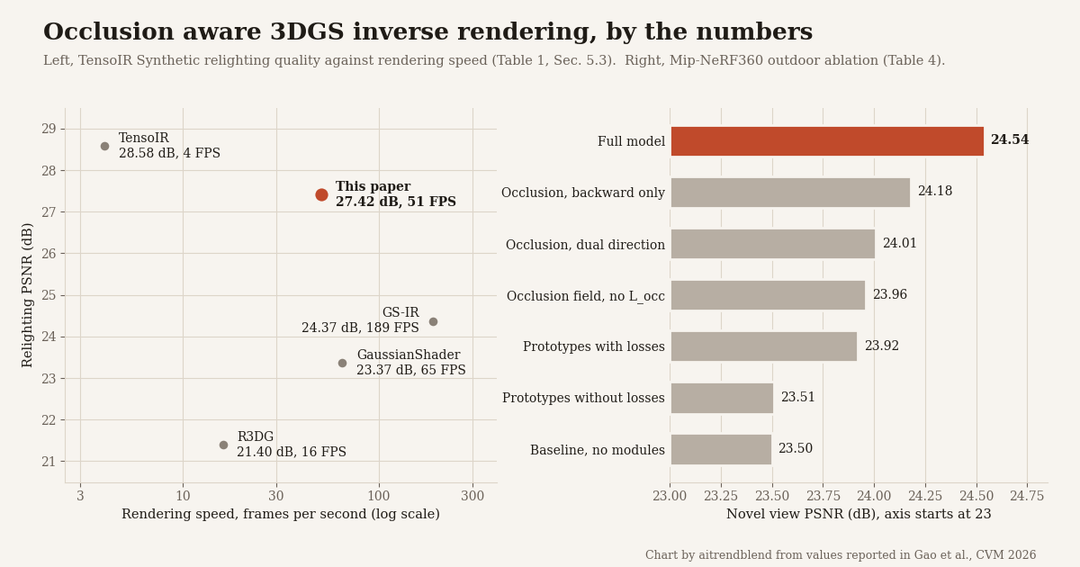
- On the TensoIR Synthetic benchmark the method leads all 3DGS pipelines on novel view synthesis (38.05 dB) and relighting (27.42 dB) while running at 51 frames per second after about an hour of training.
- A NeRF based method, TensoIR, still relights more accurately on PSNR and SSIM, and on real unbounded scenes plain 3DGS matches or beats it on view synthesis. Gains are real but targeted.
Why relighting a splatted scene is harder than rendering one
Rendering a captured scene from a new viewpoint only requires getting the pixels right. 3D Gaussian splatting does that brilliantly by fitting millions of small, semi transparent ellipsoids whose colors change with view direction, then sorting and blending them on the GPU. The color each Gaussian stores, though, is a finished product. It already contains the light that fell on the surface, the shadow cast by a neighbor, the reflection of a window. Nothing tells you which part came from the material and which came from the room.
Inverse rendering tries to split that finished color back into its ingredients. Geometry, meaning positions and surface normals. Reflectance, usually a BRDF described by albedo, metalness and roughness. Illumination, typically an HDR environment map. The trouble is that the problem is badly underdetermined. A dark patch on a wooden table might be dark wood under bright light or pale wood in shadow, and the photographs alone cannot tell you which. Every successful method leans on two things, a physically faithful model of how light reaches each point and good priors about what materials and lights usually look like.
The first of those is where occlusion enters. Whether a surface point can see the sky in a given direction decides how much ambient light it receives and whether a specular highlight shows up or gets blocked. In a ray tracer you answer that by shooting rays and checking for hits. A rasterizer never shoots rays in arbitrary directions. It projects primitives onto the screen from one camera, and that is precisely why it is fast.
The shortcuts everyone else takes, and what they cost
The NeRF era produced careful solutions. NeRFactor from Zhang and colleagues factored view dependent color into BRDF lobes plus a visibility term, NeRV from Srinivasan and colleagues learned an explicit visibility field, and TensoIR from Jin and colleagues folded one bounce of global illumination into a tensor factorized radiance field. They decompose well. They are also slow. TensoIR, the strongest of them in this paper’s comparisons, needs about five hours of training and renders at about four frames per second in the authors’ own timing.
Gaussian based methods fall into two camps. Single stage pipelines such as GaussianShader from Jiang and colleagues optimize geometry, materials and lighting together, which lets each factor correct the others, but they have no good way to model direction dependent occlusion, so shadowed regions get explained by darker albedo. Multistage pipelines go the other way. GS-IR from Liang and colleagues first fits ordinary Gaussians, freezes the geometry, bakes occlusion into a spherical harmonic volume, then solves for materials. Relightable 3D Gaussians, called R3DG in the paper’s tables, adds ray tracing on top of splats for exact shadows. Freezing geometry makes occlusion tractable, but it also means a geometry error made in stage one can never be fixed by what stage three learns about materials. Ray tracing, meanwhile, drags speed back down, and R3DG renders at 16 frames per second.
So the field sat with a familiar tradeoff. Joint optimization without proper occlusion, or proper occlusion without joint optimization. Likun Gao, Yijun Feng, Shibang Xiao and Xiaohui Liang, working at Beihang University’s State Key Laboratory of Virtual Reality Technology and Systems and at Zhongguancun Laboratory, set out to get both in one training loop. Their paper, Occlusion aware 3D Gaussian splatting for real time inverse rendering, appeared in Computational Visual Media in August 2026.
Reading occlusion off the splatting pass itself
Start with what 3DGS computes anyway. For a pixel, the Gaussians along its ray are sorted front to back. Each contributes an opacity \(\alpha_k\), and its color is weighted by the forward transmittance, how much light survives the Gaussians in front of it.
Forward transmittance tells you how visible a Gaussian is to the camera. It says nothing about how visible the environment is to the Gaussian, and it quietly assumes the space behind the camera is empty, which fails badly for indoor or unbounded captures. The authors flip the product around.
This measures how much of the ray behind Gaussian \(i\), on the far side from the camera, is empty. If nothing sits back there, \(\hat{T}_i\) is close to one and light from that direction could reach the Gaussian. If a wall or another object is back there, \(\hat{T}_i\) drops toward zero. The quantity depends only on geometry the camera has actually seen, and it is differentiable through the same compositing math, so it comes essentially for free.
Picture standing in a crowd at a concert and wanting to know whether you could see the exit behind you. You cannot turn around, but a drone overhead looking along the same line can count the people between you and the door. Each camera view is one such drone, and over many views each Gaussian collects a few dozen of these directional readings.
Twenty five numbers per Gaussian
Readings from scattered directions need somewhere to live. Each Gaussian gets a vector of occlusion coefficients on the real spherical harmonic basis up to order four, which comes to 25 numbers. Together they define a smooth visibility function over the sphere.
Training ties that field to the pseudo label with a plain binary cross entropy, evaluated along the direction the label was measured in.
At render time the backward transmittance is no longer needed. The coefficients are simply evaluated.
Why backward and not both directions
An obvious extension is to supervise the forward direction too, or both at once. The authors argue against it. Forward transmittance is conditioned on where the camera happened to stand, and in scene captures there are often occluders behind the sensor or outside every view that the model never sees. Forcing the visibility field to match those targets teaches it camera specific artifacts rather than environment visibility. Their ablation backs this up. On the outdoor Mip-NeRF 360 scenes, backward only supervision reaches 24.18 dB, while adding forward direction targets drops it to 24.01 dB.
Ambient occlusion in twenty five multiply adds
Ambient occlusion is the cosine weighted fraction of the hemisphere above a point that is not blocked. Computed by Monte Carlo sampling it is noisy and slow. Here both the visibility and the cosine lobe live on the same orthonormal SH basis, and for any fixed normal the SH coefficients of the clamped cosine are known in closed form. The authors call these normal related SH. The hemispherical integral collapses into a dot product.
That is 25 fused multiply adds per pixel. The paper does not print the normal related coefficients, but they follow from the Funk and Hecke theorem, and the eigenvalues of the clamped cosine for orders zero through four are \(\pi\), \(2\pi/3\), \(\pi/4\), \(0\) and \(-\pi/24\). The code at the end of this article uses those values and checks them numerically against brute force integration. The odd order three term vanishing exactly is a nice sanity check if you implement this yourself.
The rasterizer already multiplies transparencies along every ray. Reading that product from the far end gives each Gaussian a free, differentiable estimate of how open the scene is behind it, and a 25 coefficient SH field turns those estimates into visibility for any direction.
Materials come in a handful of flavors
The second idea addresses the other half of the ambiguity. Look at a ground truth albedo map of the Lego bulldozer and plot a histogram of its colors, as the authors do in their first figure. Instead of a smooth spread, you get a few sharp spikes. Real objects are made of a small number of materials, painted plastic, rubber, metal, and within each one the base color barely changes. Shading, by contrast, varies continuously. When an optimizer is free to give every Gaussian its own independent albedo, it can explain a soft shadow by darkening the albedo gradually, and the shadow leaks into the material.
The fix is a learned palette. A global table of \(K\) prototype colors \(\mathbf{A}_k\) is optimized together with everything else, and each Gaussian carries a probability vector over them plus a small residual.
On its own this would just be a linear mixing layer, and the ablation shows exactly that. Prototypes without extra losses score 23.51 dB against 23.50 for no prototypes at all. The work is done by two regularizers. The first is a material aggregation loss that rewards each Gaussian for committing to one prototype.
The expression inside the logarithm has a tidy interpretation. Treat each prototype as an independent coin that comes up active with probability \(p_{ik}\). The inner sum is then the probability that exactly one coin is active. The authors prove that this is at most one and equals one only when the assignment is one hot, so the loss is zero exactly at clean, single material assignments. For a sense of scale, with 32 prototypes and a perfectly uniform assignment the per Gaussian loss works out to about 0.98, which our code confirms. The paper is careful to say this establishes where the minima are, not that gradient descent will reach them.
The second regularizer, an L1 penalty on the residual, lets prototypes carry the dominant colors while the residual handles texture, wear and anything the palette cannot express. The residual really does stay small. Measured as a fraction of the total albedo norm it comes to 7.4 percent on Lego, 8.0 percent on the indoor Bonsai scene and 4.7 percent on the outdoor Bicycle scene.
Readers who follow our coverage of entropy based surface priors for Gaussians will recognize the pattern. A soft, well motivated prior on what the scene should look like steers an underdetermined optimization without hard constraints.
Putting it together in a deferred split sum shader
Shading every Gaussian and then blending the results, forward shading, would mix lighting from many primitives per pixel. The method instead uses deferred shading. A first pass splats per Gaussian attributes into screen space buffers, normals, albedo, metalness, roughness and the 25 occlusion coefficients. A second pass shades each pixel once, using a Disney style microfacet BRDF with a Lambertian diffuse lobe and a GGX specular lobe.
For speed, the specular integral uses the split sum approximation popularized by Brian Karis for Unreal Engine 4. The environment is prefiltered by roughness into a mip chain, the BRDF part is integrated into a two dimensional lookup table indexed by roughness and viewing angle, and specular shading reduces to a couple of texture fetches. The learned visibility slots straight into this.
Ambient occlusion darkens the diffuse term. For specular light, the visibility along the reflection direction \(R\) decides how much comes from the environment map and how much from an indirect term. That indirect term borrows an idea from GS-IR. Each Gaussian holds 16 more SH coefficients, third order this time, which weight the low frequency environment radiance sampled at 32 fixed directions spread over the sphere. It is a crude stand in for interreflection, but it is cheap and differentiable.
The full objective balances six terms.
The image term is mean absolute error plus D-SSIM. The lighting term penalizes each environment texel for deviating from its own channel average, nudging the recovered light toward neutral white so that color casts get attributed to materials rather than to a tinted sky. The smoothness term is edge aware, applied to metalness, roughness and normals, and relaxed wherever the photograph itself has a strong edge. Training runs for about 30,000 iterations with Adam, learning rate 0.002 for geometry and 0.001 for appearance, halved every 20,000 iterations, on a single RTX 4090. The prototype count is preset to 32 for every dataset.
One detail the paper leaves out is the value of each \(\lambda\). Anyone reproducing the work will need to tune them, and the balance between \(\mathcal{L}_{\mathrm{occ}}\) and the image loss in particular will shape how the visibility field behaves.
What the numbers say
Object level decomposition
TensoIR Synthetic is the standard benchmark here, four Blender objects with ground truth normals, albedo and relit images. The table below reproduces the paper’s results.
| Method | Normal MAE ↓ | NVS PSNR ↑ | NVS SSIM ↑ | NVS LPIPS ↓ | Relight PSNR ↑ | Relight SSIM ↑ | Relight LPIPS ↓ | Family |
|---|---|---|---|---|---|---|---|---|
| NeRFactor | 6.314 | 24.679 | 0.922 | 0.120 | 23.383 | 0.908 | 0.131 | NeRF |
| InvRender | 5.074 | 27.367 | 0.934 | 0.089 | 23.973 | 0.901 | 0.101 | NeRF |
| NVDiffrec | 6.078 | 30.696 | 0.962 | 0.052 | 19.880 | 0.879 | 0.104 | NeRF |
| TensoIR | 4.100 | 35.088 | 0.976 | 0.040 | 28.580 | 0.944 | 0.081 | NeRF |
| GS-IR | 4.948 | 35.333 | 0.974 | 0.039 | 24.374 | 0.885 | 0.096 | 3DGS |
| GaussianShader | 6.525 | 37.573 | 0.984 | 0.022 | 23.372 | 0.874 | 0.105 | 3DGS |
| R3DG | 4.728 | 37.131 | 0.984 | 0.022 | 21.404 | 0.860 | 0.127 | 3DGS |
| This paper | 4.215 | 38.049 | 0.986 | 0.020 | 27.424 | 0.923 | 0.068 | 3DGS |
Table 1 of the paper, TensoIR Synthetic. NVS stands for novel view synthesis. Normal error is mean angular error.
Among Gaussian methods the new pipeline wins every column, and the relighting jump is the headline. It gains over 3 dB on GS-IR and about 4 dB on GaussianShader. Novel view synthesis also improves slightly, which is not guaranteed for inverse rendering methods, since a physically constrained shader often gives up a little image fidelity compared with free view dependent color. Relighting LPIPS, at 0.068, is the best of any method in the table.
TensoIR still holds the best normals and the best relighting PSNR and SSIM. The gap is about 1.2 dB in relighting PSNR. For a method that trains five times faster and renders more than twelve times faster, that is a respectable place to land, but it is not a clean sweep, and the paper’s table marks it honestly.
On the Shiny Blender dataset, built to stress glossy and mirror like surfaces, the method averages 31.83 dB on novel view synthesis. That is ahead of GaussianShader by 1.17 dB, Relightable 3DGS by 3.65 dB and GS-IR by 5.48 dB, and slightly ahead of the NeRF based NeRO at 30.83 dB. It ranks first among Gaussian methods on five of six objects, losing only on the Teapot, where Relightable 3DGS scores 43.59 dB against 42.98.
Real scenes, read closely
The real world results deserve a slower read than the bold numbers invite.
| Method | Outdoor PSNR | Outdoor SSIM | Outdoor LPIPS | Indoor PSNR | Indoor SSIM | Indoor LPIPS | Ref-NeRF PSNR | Ref-NeRF SSIM | Ref-NeRF LPIPS |
|---|---|---|---|---|---|---|---|---|---|
| Mip-NeRF 360 | 24.43 | 0.694 | 0.278 | 31.49 | 0.918 | 0.179 | 24.27 | 0.649 | 0.276 |
| UniSDF | 24.77 | 0.723 | 0.241 | 31.28 | 0.901 | 0.181 | 23.70 | 0.635 | 0.266 |
| 3DGS | 24.64 | 0.731 | 0.234 | 30.41 | 0.917 | 0.190 | 23.67 | 0.632 | 0.288 |
| 2DGS | 24.33 | 0.709 | 0.284 | 30.39 | 0.922 | 0.183 | 23.65 | 0.634 | 0.285 |
| GS-IR | 23.45 | 0.671 | 0.284 | 27.80 | 0.870 | 0.248 | 23.32 | 0.625 | 0.283 |
| GaussianShader | 22.80 | 0.665 | 0.297 | 26.61 | 0.878 | 0.243 | 22.96 | 0.624 | 0.294 |
| GUS-IR | 23.76 | 0.696 | 0.276 | 28.98 | 0.902 | 0.222 | 23.67 | 0.646 | 0.282 |
| This paper | 24.54 | 0.728 | 0.231 | 31.17 | 0.916 | 0.195 | 23.81 | 0.656 | 0.280 |
Table 2 of the paper. The first four rows are reconstruction methods that do not decompose materials or lighting. The last four are 3DGS inverse rendering methods.
Against the other inverse rendering methods the margin is large, about 0.8 dB over GUS-IR outdoors and more than 2 dB indoors. Against pure reconstruction methods, the story changes. Plain 3DGS scores 24.64 dB outdoors against 24.54, and Mip-NeRF 360 scores 31.49 dB indoors against 31.17. The abstract says the approach stays competitive with strong reconstruction baselines, and that is the accurate phrasing. What you get is a decomposed, relightable scene at close to the view quality of a model that does not decompose anything. That is the real selling point. Anyone expecting better novel view synthesis than vanilla 3DGS on real scenes will not find it here.
Speed
Under a fixed hardware and resolution setup on TensoIR Synthetic, the paper reports training time and frame rate for each method. TensoIR takes 5 hours and renders at 4 FPS. GS-IR takes 0.4 hours and runs at 189 FPS. GaussianShader takes an hour at 65 FPS. R3DG takes an hour at 16 FPS. The new method takes about an hour and runs at 51 FPS. The occlusion field costs something, 25 extra scalars per Gaussian plus the prototype vector and residual, and the method gives up roughly three quarters of GS-IR’s frame rate in exchange for about 3 dB of relighting quality. The paper does not state the rendering resolution behind those figures, so comparisons with numbers from other papers should be made with care.
What the ablations reveal
| Configuration | PSNR ↑ | SSIM ↑ | LPIPS ↓ |
|---|---|---|---|
| Baseline, neither module | 23.50 | 0.686 | 0.280 |
| Occlusion field, no occlusion loss | 23.96 | 0.706 | 0.265 |
| Learnable occlusion, backward supervision | 24.18 | 0.720 | 0.244 |
| Learnable occlusion, dual direction supervision | 24.01 | 0.712 | 0.256 |
| Prototypes, no losses | 23.51 | 0.688 | 0.288 |
| Prototypes with aggregation and residual losses | 23.92 | 0.704 | 0.268 |
| Full model | 24.54 | 0.728 | 0.231 |
Table 4 of the paper, outdoor Mip-NeRF 360 scenes.
Three things stand out. The occlusion field helps even without its dedicated loss, from 23.50 to 23.96 dB, because the photometric gradient alone gives it something to fit. The pseudo label adds another 0.22 dB and visibly cleaner occlusion maps, with leaf surfaces correctly marked as open rather than shadowed. And the two modules stack almost additively. Occlusion alone adds 0.68 dB, prototypes alone add 0.42 dB, both together add 1.04 dB. That near additivity suggests they fix different failure modes, which is exactly what the design intends.
The SH order study is equally clean. Third order visibility with 16 coefficients gives 24.31 dB, fourth order with 25 gives 24.54, fifth with 36 gives 24.58 and sixth with 49 gives 24.59. Visibility in these scenes is dominated by low frequency structure, and the default of order four is a sensible place to stop.
“Backward transmittance and directional visibility are physically equivalent quantities under the volumetric rendering model.”Gao, Feng, Xiao and Liang, Computational Visual Media, 2026
Where we would push back
The backward transmittance idea is elegant, and the ablation says it helps. It is still worth asking which directions it actually supervises. Think about a Gaussian on the front face of a solid object. The stretch of ray behind it runs straight into the object’s own interior, so the pseudo label for that direction is near zero. That is correct, but it concerns a direction below the surface, which the cosine weighted ambient occlusion integral ignores. The hemisphere facing the camera, the one that matters for shading, rarely receives a direct label from this mechanism unless the geometry is thin, like leaves, or the view grazes a concave region.
Our reading is that much of the visible hemisphere is shaped by the photometric loss flowing back through the shader, with the pseudo label anchoring the low order coefficients that both hemispheres share. This is an interpretation, not something the paper measures. Since TensoIR Synthetic provides exact geometry, a direct comparison of learned visibility against ray traced visibility would settle the question and would be a welcome addition to future versions of this work.
A few smaller points. The text describes the residual as accounting for 5 to 8 percent of the final albedo, while the table beside it lists 4.7 percent for Bicycle, a trivial mismatch but one a careful reader will notice. Loss weights are not reported. We could not find a public code release linked to the paper at the time of writing, so reproducing the exact numbers means rebuilding the pipeline. And the prototype count is fixed at 32 per dataset, which works for the benchmarks but leaves open how the method behaves when a scene contains many more distinct materials than that.
Treat this as the best Gaussian based relighting pipeline in its comparison set rather than a replacement for either ray traced inverse rendering or vanilla 3DGS. It closes most of the relighting gap to TensoIR at interactive speed, and it keeps real scene view quality close to plain 3DGS while also giving you materials and lighting.
Limitations the authors acknowledge
The paper closes with an unusually specific limitations section, and each item is worth taking seriously.
Material prior expressiveness. Prototypes assume a scene’s reflectance can be roughly explained by a small set of colors. In scenes with highly varied, spatially continuous or finely detailed materials, the residual has to carry more of the appearance, the prototype assignments become harder to interpret, and the separation between material and light can weaken. The authors suggest richer prototype parameterizations or learned spatial regularizers as next steps.
Static scenes only. The visibility field is learned from transmittance under one fixed configuration of the scene. Move an object and the stored coefficients describe a world that no longer exists. Extending the idea to dynamic content would need explicit temporal modeling, for example deformation fields or time dependent visibility. For readers following rigged and animated Gaussian models, this is the obvious gap to watch.
Approximate light transport. Split sum shading with simplified visibility and one low frequency indirect term is not full global illumination. Structured indoor lighting, strong interreflections, sharp cast shadows and caustics can still bleed color into albedo, oversmooth normals on thin structures and soften contact shadows. This is a limitation shared by every real time PBR inverse renderer, and the paper says so directly. For readers who want to see what exact light transport requires, our piece on sampling volumetric emitters in Monte Carlo rendering shows the other end of the speed and accuracy spectrum.
Who should care about this
The obvious audience is anyone turning captures into assets. Film and game pipelines want scanned props that behave correctly under new lighting, and they want them in hours rather than days. An hour of training on one consumer GPU, with relighting quality within about 1.2 dB of a five hour NeRF method, moves Gaussian captures closer to that bar. Tools like the ones in our Luma AI scene capture guide already produce splats that look good in place. Making them relightable is the step that lets them leave the room they were captured in.
Augmented reality benefits for the same reason. Placing a scanned object into a live camera feed only looks right if it picks up the real room’s lighting, which requires separated albedo and lighting in the first place. Robotics simulation is a third customer. Physically consistent digital twins let perception models train under many lighting conditions without recapturing the environment each time.
The broader lesson travels further. Rasterization pipelines throw away a lot of information that turns out to be useful. Backward transmittance was sitting in every 3DGS forward pass the whole time. Similar tricks may turn up elsewhere, for instance in the occlusion reasoning that point trackers need or in generative pipelines that must place objects with plausible shadows, the problem behind DreamFuse’s diffusion based image fusion. For more 3D vision work on the site, the computer vision archive collects the Gaussian splatting cluster in one place.
Reference implementation in PyTorch
The code below implements every component described in the paper in a single file. It contains a gradient safe real SH basis up to order four, a dense and fully differentiable splatting rasterizer that returns both forward and backward transmittance, the occlusion field with its pseudo label loss, ambient occlusion through normal related SH, the 32 direction indirect term, prototype albedo with aggregation and residual losses, a split sum shader with a learnable HDR environment and a Monte Carlo BRDF lookup table, the six term objective, the optimizer schedule from the paper, evaluation, relighting and a smoke test.
Two honest caveats. The dense rasterizer evaluates every Gaussian at every pixel, which is fine for a toy scene and hopeless for a real capture, so for real data keep the losses and shader and replace the rasterize method with a tiled CUDA rasterizer such as the one in gsplat. And because the paper does not report loss weights, the values in LAMBDAS are our own starting points, and the sigmoid on the occlusion field follows our reading of the paper’s pipeline figure.
"""
Occlusion-aware 3D Gaussian splatting for real-time inverse rendering.
Reference PyTorch implementation of the ideas in
    Gao, Feng, Xiao, Liang. Computational Visual Media 12(4), 989-1007, 2026.
    https://doi.org/10.26599/CVM.2026.9450563

What this file contains
    * real spherical harmonics up to order 4 (25 coefficients), gradient safe
    * a dense, fully differentiable Gaussian splatting rasterizer in pure PyTorch
      that returns BOTH forward transmittance T_k and backward transmittance T_hat_k
    * per-Gaussian occlusion SH (25 coeffs) supervised by backward-transmittance
      pseudo labels (Eq. 14-15)
    * ambient occlusion by a 25-term dot product with normal-related SH (Eq. 16-18)
    * low-frequency indirect light from 16 SH coefficients and 32 fixed directions (Eq. 19-20)
    * prototype-based albedo, aggregation loss and residual sparsity (Eq. 23-25)
    * deferred split-sum PBR shading with a learnable HDR environment (Eq. 21-22)
    * the six-term objective of Eq. 29, training loop, evaluation and relighting

What it is not
    The dense rasterizer evaluates every Gaussian at every pixel, so it is meant for
    small scenes, teaching and unit testing. For real captures, keep the loss and shading
    code and swap `rasterize` for a tiled CUDA rasterizer such as gsplat or the official
    3DGS one. Densification and pruning from vanilla 3DGS are omitted for the same reason.
    Loss weights are not reported in the paper; the defaults below are our starting values.
"""
import math
import torch
import torch.nn as nn
import torch.nn.functional as F

# ---------------------------------------------------------------------------
# 1. Real spherical harmonics (orthonormal), any order, gradient safe at poles
# ---------------------------------------------------------------------------

def real_sh(dirs: torch.Tensor, lmax: int) -> torch.Tensor:
    """dirs (..., 3) unit vectors -> (..., (lmax+1)^2) real SH values.
    Index of (l, m) is l*l + l + m. Uses P_l^m / sin^m(theta) recurrences multiplied by
    Re/Im((x + i y)^m) so no atan2 is involved and gradients stay finite at the poles."""
    x, y, z = dirs[..., 0], dirs[..., 1], dirs[..., 2]
    out = [None] * ((lmax + 1) ** 2)
    # A_m = Re((x+iy)^m), B_m = Im((x+iy)^m)
    A, B = [torch.ones_like(x)], [torch.zeros_like(x)]
    for m in range(1, lmax + 1):
        A.append(x * A[m - 1] - y * B[m - 1])
        B.append(x * B[m - 1] + y * A[m - 1])
    for m in range(0, lmax + 1):
        # Q_m^m = (-1)^m (2m-1)!!
        dfact = 1.0
        for k in range(1, 2 * m, 2):
            dfact *= k
        Q = {m: torch.full_like(z, ((-1.0) ** m) * dfact)}
        if m + 1 <= lmax:
            Q[m + 1] = z * (2 * m + 1) * Q[m]
        for l in range(m + 2, lmax + 1):
            Q[l] = ((2 * l - 1) * z * Q[l - 1] - (l + m - 1) * Q[l - 2]) / (l - m)
        for l in range(m, lmax + 1):
            K = math.sqrt((2 * l + 1) / (4 * math.pi) * math.factorial(l - m) / math.factorial(l + m))
            if m == 0:
                out[l * l + l] = K * Q[l]
            else:
                out[l * l + l + m] = math.sqrt(2.0) * K * Q[l] * A[m]
                out[l * l + l - m] = math.sqrt(2.0) * K * Q[l] * B[m]
    return torch.stack(out, dim=-1)


# Funk-Hecke eigenvalues of the clamped cosine kernel max(0, n.w) for l = 0..4.
# Projecting (n.w)+ onto SH gives c_lm^NRSH(n) = lambda_l * Y_lm(n)   (Eq. 17)
CLAMPED_COS_EIG = torch.tensor([math.pi, 2 * math.pi / 3, math.pi / 4, 0.0, -math.pi / 24])


def nrsh(normals: torch.Tensor) -> torch.Tensor:
    """Normal-related SH, (..., 25). Includes the 1/pi of Eq. 16 so AO = <c_occ, nrsh>."""
    lam = CLAMPED_COS_EIG.to(normals)
    per_coeff = torch.cat([lam[l].repeat(2 * l + 1) for l in range(5)])
    return real_sh(normals, 4) * per_coeff / math.pi


def fibonacci_sphere(n: int) -> torch.Tensor:
    i = torch.arange(n, dtype=torch.float32) + 0.5
    phi = torch.acos(1 - 2 * i / n)
    theta = math.pi * (1 + 5 ** 0.5) * i
    return torch.stack([torch.cos(theta) * torch.sin(phi),
                        torch.sin(theta) * torch.sin(phi),
                        torch.cos(phi)], -1)


# ---------------------------------------------------------------------------
# 2. Camera and environment helpers
# ---------------------------------------------------------------------------

class Camera:
    def __init__(self, eye, target, H, W, fov_deg=45.0, up=(0.0, 0.0, 1.0)):
        eye, target, up = map(lambda v: torch.tensor(v, dtype=torch.float32), (eye, target, up))
        f = F.normalize(target - eye, dim=0)
        r = F.normalize(torch.linalg.cross(f, up), dim=0)
        u = torch.linalg.cross(r, f)
        # world -> camera, camera looks down +z, x right, y down (OpenCV style)
        self.R = torch.stack([r, -u, f], 0)
        self.t = -self.R @ eye
        self.center = eye
        self.H, self.W = H, W
        self.fx = self.fy = 0.5 * W / math.tan(math.radians(fov_deg) / 2)
        self.cx, self.cy = W / 2, H / 2

    def pixel_grid(self):
        ys, xs = torch.meshgrid(torch.arange(self.H) + 0.5, torch.arange(self.W) + 0.5, indexing="ij")
        return torch.stack([xs, ys], -1).reshape(-1, 2)

    def ray_dirs(self):
        pix = self.pixel_grid()
        d_cam = torch.stack([(pix[:, 0] - self.cx) / self.fx, (pix[:, 1] - self.cy) / self.fy,
                             torch.ones(len(pix))], -1)
        return F.normalize(d_cam @ self.R, dim=-1)  # R^T d  in world space


def equirect_dirs(He, We):
    v, u = torch.meshgrid((torch.arange(He) + 0.5) / He, (torch.arange(We) + 0.5) / We, indexing="ij")
    theta, phi = v * math.pi, u * 2 * math.pi
    d = torch.stack([torch.sin(theta) * torch.cos(phi), torch.sin(theta) * torch.sin(phi), torch.cos(theta)], -1)
    d_omega = (math.pi / He) * (2 * math.pi / We) * torch.sin(theta)
    return d.reshape(-1, 3), d_omega.reshape(-1)


def ggx_D(cos_h, alpha):
    a2 = alpha ** 2
    denom = cos_h ** 2 * (a2 - 1) + 1
    return a2 / (math.pi * denom ** 2 + 1e-8)


def build_brdf_lut(res=32, samples=512):
    """Split-sum 2D LUT (Karis 2013). Returns (2, res, res) indexed [channel, roughness, NoV]."""
    nov = (torch.arange(res) + 0.5) / res
    rough = (torch.arange(res) + 0.5) / res
    NoV, Rg = torch.meshgrid(nov, rough, indexing="xy")          # (res, res) rows=rough
    i = torch.arange(samples, dtype=torch.float32)
    u1 = (i + 0.5) / samples
    bits = torch.tensor([int(f"{k:032b}"[::-1], 2) for k in range(samples)], dtype=torch.float64)
    u2 = (bits / 2 ** 32).float()                                 # Hammersley
    a = (Rg ** 2)[..., None]
    phi = 2 * math.pi * u1
    cos_t = torch.sqrt((1 - u2) / (1 + (a ** 2 - 1) * u2))
    sin_t = torch.sqrt(1 - cos_t ** 2)
    H = torch.stack([sin_t * torch.cos(phi).expand_as(sin_t), sin_t * torch.sin(phi).expand_as(sin_t), cos_t], -1)
    V = torch.stack([torch.sqrt(1 - NoV ** 2), torch.zeros_like(NoV), NoV], -1)[..., None, :]
    VoH = (V * H).sum(-1)
    L = 2 * VoH[..., None] * H - V
    NoL, NoH = L[..., 2].clamp(min=0), H[..., 2].clamp(min=0)
    k = a / 2
    nv = NoV[..., None]
    G = (nv / (nv * (1 - k) + k)) * (NoL / (NoL * (1 - k) + k))
    G_vis = G * VoH.clamp(min=0) / (NoH * nv + 1e-8)
    Fc = (1 - VoH.clamp(min=0)) ** 5
    valid = (NoL > 0).float()
    A = ((1 - Fc) * G_vis * valid).mean(-1)
    Bv = (Fc * G_vis * valid).mean(-1)
    return torch.stack([A, Bv], 0)


# ---------------------------------------------------------------------------
# 3. The model: Gaussians with occlusion SH, prototype albedo and PBR attributes
# ---------------------------------------------------------------------------

class OcclusionAwareGaussians(nn.Module):
    def __init__(self, n=512, K=32, env_res=(16, 32), extent=1.0, seed=0):
        super().__init__()
        g = torch.Generator().manual_seed(seed)
        self.K = K
        # geometry
        self.means = nn.Parameter((torch.rand(n, 3, generator=g) - 0.5) * 2 * extent)
        self.log_scales = nn.Parameter(torch.full((n, 3), math.log(0.08 * extent)) + 0.2 * torch.randn(n, 3, generator=g))
        self.quats = nn.Parameter(F.normalize(torch.randn(n, 4, generator=g), dim=-1))
        self.opacity_logit = nn.Parameter(torch.full((n, 1), 0.5))
        self.normals_raw = nn.Parameter(F.normalize(torch.randn(n, 3, generator=g), dim=-1))
        # material
        self.metal_logit = nn.Parameter(torch.full((n, 1), -2.0))
        self.rough_logit = nn.Parameter(torch.zeros(n, 1))
        self.proto_logits = nn.Parameter(0.01 * torch.randn(n, K, generator=g))   # p_i on the simplex
        self.prototypes = nn.Parameter(torch.rand(K, 3, generator=g))            # A_k, random init
        self.residual = nn.Parameter(0.01 * torch.randn(n, 3, generator=g))      # eps_i, random init
        # visibility and indirect light
        self.occ_sh = nn.Parameter(torch.zeros(n, 25))                            # c^occ, 4th order
        self.occ_sh.data[:, 0] = 2.0 / 0.2820948                                  # start near "visible"
        self.ind_sh = nn.Parameter(torch.zeros(n, 16))                            # c^ind, 3rd order
        # learnable HDR environment (equirectangular, softplus to stay positive)
        self.env_raw = nn.Parameter(torch.full((*env_res, 3), 0.5) + 0.05 * torch.randn(*env_res, 3, generator=g))
        env_dirs, env_dw = equirect_dirs(*env_res)
        self.register_buffer("env_dirs", env_dirs)
        self.register_buffer("env_dw", env_dw)
        self.register_buffer("brdf_lut", build_brdf_lut())
        self.register_buffer("ind_dirs", fibonacci_sphere(32))                    # N_dir = 32
        self.register_buffer("ind_Y", real_sh(fibonacci_sphere(32), 3))           # (32, 16)

    # --- attribute accessors ---
    def opacity(self):
        return torch.sigmoid(self.opacity_logit)

    def proto_probs(self):
        return torch.softmax(self.proto_logits, -1)

    def albedo(self):
        """Eq. 23: a_i = sum_k p_ik A_k + eps_i."""
        base = self.proto_probs() @ self.prototypes.clamp(0, 1)
        return (base + self.residual).clamp(0, 1)

    def env(self):
        return F.softplus(self.env_raw).reshape(-1, 3)

    def covariances(self):
        q = F.normalize(self.quats, dim=-1)
        w, x, y, z = q.unbind(-1)
        R = torch.stack([1 - 2 * (y * y + z * z), 2 * (x * y - w * z), 2 * (x * z + w * y),
                         2 * (x * y + w * z), 1 - 2 * (x * x + z * z), 2 * (y * z - w * x),
                         2 * (x * z - w * y), 2 * (y * z + w * x), 1 - 2 * (x * x + y * y)], -1).view(-1, 3, 3)
        S = torch.diag_embed(torch.exp(self.log_scales))
        M = R @ S
        return M @ M.transpose(1, 2)                                              # Eq. 1

    # --- rasterizer ---
    def rasterize(self, cam: Camera, attrs: torch.Tensor):
        """Dense front-to-back alpha compositing.
        Returns composited attrs (P, C), weights w=T*alpha (P, N_vis), forward T, backward T_hat,
        accumulated alpha and indices of visible Gaussians in depth order."""
        mu_c = self.means @ cam.R.T + cam.t
        vis = mu_c[:, 2] > 0.05
        idx = torch.nonzero(vis).squeeze(1)
        idx = idx[torch.argsort(mu_c[idx, 2])]                                    # front to back
        m = mu_c[idx]
        z = m[:, 2]
        uv = torch.stack([cam.fx * m[:, 0] / z + cam.cx, cam.fy * m[:, 1] / z + cam.cy], -1)
        J = torch.zeros(len(idx), 2, 3)
        J[:, 0, 0] = cam.fx / z
        J[:, 0, 2] = -cam.fx * m[:, 0] / z ** 2
        J[:, 1, 1] = cam.fy / z
        J[:, 1, 2] = -cam.fy * m[:, 1] / z ** 2
        cov_c = cam.R @ self.covariances()[idx] @ cam.R.T
        cov2d = J @ cov_c @ J.transpose(1, 2) + 0.3 * torch.eye(2)                # low-pass as in 3DGS
        inv = torch.linalg.inv(cov2d)
        d = cam.pixel_grid()[:, None, :] - uv[None]                               # (P, N, 2)
        power = -0.5 * torch.einsum("pni,nij,pnj->pn", d, inv, d)
        alpha = (self.opacity()[idx, 0][None] * torch.exp(power.clamp(max=0))).clamp(max=0.99)  # Eq. 3
        alpha = alpha * (alpha > 1 / 255).float()
        one_minus = 1 - alpha
        ones = torch.ones_like(alpha[:, :1])
        T = torch.cumprod(torch.cat([ones, one_minus[:, :-1]], 1), 1)             # Eq. 4, prod_{j<k}
        rev = torch.flip(one_minus, [1])
        T_hat = torch.flip(torch.cumprod(torch.cat([ones, rev[:, :-1]], 1), 1), [1])  # Eq. 14, prod_{j>k}
        w = T * alpha                                                              # Eq. 5 weights
        out = w @ attrs[idx]
        return out, w, T, T_hat, w.sum(1, keepdim=True), idx

    # --- shading pieces ---
    def diffuse_irradiance(self, n):
        """Eq. 7, L_diff(n) = int L_i(w) (w.n)+ dw, by quadrature over environment texels."""
        cos = (n @ self.env_dirs.T).clamp(min=0)
        return (cos * self.env_dw) @ self.env()

    def prefiltered(self, R, rough):
        """Split-sum prefiltered radiance L_prefilter(r, R): GGX lobe around R, normalized."""
        cos = (R @ self.env_dirs.T).clamp(min=0)
        wts = ggx_D(cos, (rough ** 2).clamp(min=0.02)) * cos * self.env_dw
        return (wts @ self.env()) / (wts.sum(-1, keepdim=True) + 1e-8)

    def lut(self, nov, rough):
        grid = torch.stack([nov * 2 - 1, rough * 2 - 1], -1).view(1, -1, 1, 2)
        s = F.grid_sample(self.brdf_lut[None], grid, align_corners=False, padding_mode="border")
        return s[0, :, :, 0].T                                                    # (P, 2)

    def render(self, cam: Camera, bg=1.0, env_override=None):
        if env_override is not None:
            saved = self.env_raw.data.clone()
            self.env_raw.data = env_override
        n_g = F.normalize(self.normals_raw, dim=-1)
        a_g = self.albedo()
        m_g, r_g = torch.sigmoid(self.metal_logit), torch.sigmoid(self.rough_logit)
        attrs = torch.cat([n_g, a_g, m_g, r_g, self.occ_sh, self.ind_sh], -1)     # 3+3+1+1+25+16 = 49
        buf, w, T, T_hat, acc, idx = self.rasterize(cam, attrs)
        # G-buffers (normalize by accumulated alpha so partially covered pixels keep sensible values)
        buf_n = buf / acc.clamp(min=1e-6)
        I_n = F.normalize(buf_n[:, 0:3], dim=-1)
        I_a, I_m, I_r = buf_n[:, 3:6], buf_n[:, 6:7], buf_n[:, 7:8]
        I_occ, I_ind = buf_n[:, 8:33], buf_n[:, 33:49]
        # deferred split-sum shading, Eq. 21-22
        v = -cam.ray_dirs()
        n_dot_v = (I_n * v).sum(-1, keepdim=True)
        I_n = torch.where(n_dot_v < 0, -I_n, I_n)                                 # face the camera
        n_dot_v = n_dot_v.abs().clamp(1e-4, 1)
        R = F.normalize(2 * n_dot_v * I_n - v, dim=-1)
        ao = torch.sigmoid((I_occ * nrsh(I_n)).sum(-1, keepdim=True))              # Eq. 18, sigmoid as in Fig. 2
        V_R = torch.sigmoid((I_occ * real_sh(R, 4)).sum(-1, keepdim=True))        # V(R), Eq. 13
        w_s = I_ind @ self.ind_Y.T                                                # Eq. 19, (P, 32)
        L_env_low = self.prefiltered(self.ind_dirs, torch.ones(32, 1))            # low-frequency env
        L_ind = (w_s @ L_env_low) / 32.0                                          # Eq. 20
        c_diff = ao * I_a * (1 - I_m) / math.pi * self.diffuse_irradiance(I_n)    # Eq. 21
        F0 = 0.04 * (1 - I_m) + I_a * I_m
        ab = self.lut(n_dot_v[:, 0], I_r[:, 0])
        spec_light = V_R * self.prefiltered(R, I_r) + (1 - V_R) * L_ind
        c_spec = spec_light * (F0 * ab[:, :1] + ab[:, 1:2])                       # Eq. 22
        rgb_lin = c_diff + c_spec
        rgb = rgb_lin.clamp(0, 1) * acc + bg * (1 - acc)
        if env_override is not None:
            self.env_raw.data = saved
        H, W = cam.H, cam.W
        return {
            "rgb": rgb.view(H, W, 3), "normal": I_n.view(H, W, 3), "albedo": I_a.view(H, W, 3),
            "metal": I_m.view(H, W, 1), "rough": I_r.view(H, W, 1), "ao": ao.view(H, W, 1),
            "alpha": acc.view(H, W, 1), "w": w, "T_hat": T_hat, "idx": idx,
        }


# ---------------------------------------------------------------------------
# 4. Losses (Eq. 15, 24, 25, 29-32)
# ---------------------------------------------------------------------------

def occlusion_loss(model: OcclusionAwareGaussians, cam: Camera, out):
    """Eq. 15. Pseudo label p_hat_i = backward transmittance T_hat_i, averaged over the pixels
    that Gaussian i actually contributes to (weights w = T*alpha), detached.
    Query direction: the continuation of the view ray past the Gaussian, i.e. the side of the
    scene that the Gaussians j > i occupy. The paper names this w_b = -w_f using a light
    propagation convention; as a lookup direction toward the light it is this vector."""
    w, T_hat, idx = out["w"], out["T_hat"], out["idx"]
    wsum = w.sum(0)
    keep = wsum > 1e-3
    if keep.sum() == 0:
        return torch.zeros(())
    p_hat = ((w * T_hat).sum(0) / wsum.clamp(min=1e-8)).detach()
    d = F.normalize(model.means[idx] - cam.center, dim=-1).detach()
    logit = (model.occ_sh[idx] * real_sh(d, 4)).sum(-1)
    return F.binary_cross_entropy_with_logits(logit[keep], p_hat[keep])


def aggregation_loss(p: torch.Tensor, eps=1e-6):
    """Eq. 24/26/27. Q_i = sum_k p_ik prod_{j!=k}(1-p_ij), probability of exactly one active
    prototype. L_agg = -sum_i log Q_i, zero iff every p_i is one-hot. We average over i."""
    log1m = torch.log((1 - p).clamp(min=eps))
    prod_except = torch.exp(log1m.sum(-1, keepdim=True) - log1m)
    Q = (p * prod_except).sum(-1)
    return -torch.log(Q.clamp(min=eps)).mean()


def residual_sparsity(eps_res: torch.Tensor):
    """Eq. 25, ||eps_i||_1 (mean over Gaussians; lambda_res absorbs the scale)."""
    return eps_res.abs().sum(-1).mean()


def light_neutrality(env: torch.Tensor):
    """Eq. 31, mean absolute deviation of each texel's channels from their channel mean."""
    return (env - env.mean(-1, keepdim=True)).abs().mean()


def edge_aware_smooth(x: torch.Tensor, img: torch.Tensor):
    """Eq. 32 on an (H, W, C) G-buffer guided by the (H, W, 3) reference image."""
    dx_x = (x[:, 1:] - x[:, :-1]).abs().mean(-1)
    dy_x = (x[1:] - x[:-1]).abs().mean(-1)
    dx_i = (img[:, 1:] - img[:, :-1]).abs().mean(-1)
    dy_i = (img[1:] - img[:-1]).abs().mean(-1)
    return (dx_x * torch.exp(-dx_i)).mean() + (dy_x * torch.exp(-dy_i)).mean()


def ssim(a: torch.Tensor, b: torch.Tensor, win=7):
    """a, b: (H, W, 3) in [0, 1]."""
    a, b = a.permute(2, 0, 1)[None], b.permute(2, 0, 1)[None]
    g = torch.exp(-((torch.arange(win) - win // 2) ** 2) / (2 * 1.5 ** 2))
    g = (g / g.sum())
    k = (g[:, None] * g[None]).expand(3, 1, win, win)
    f = lambda t: F.conv2d(t, k, padding=win // 2, groups=3)
    mu_a, mu_b = f(a), f(b)
    s_aa, s_bb, s_ab = f(a * a) - mu_a ** 2, f(b * b) - mu_b ** 2, f(a * b) - mu_a * mu_b
    C1, C2 = 0.01 ** 2, 0.03 ** 2
    m = ((2 * mu_a * mu_b + C1) * (2 * s_ab + C2)) / ((mu_a ** 2 + mu_b ** 2 + C1) * (s_aa + s_bb + C2))
    return m.mean()


def psnr(a, b):
    return -10 * torch.log10(F.mse_loss(a, b).clamp(min=1e-10))


LAMBDAS = dict(img=1.0, l=0.01, s=0.01, occ=0.1, agg=0.01, res=0.01)  # not reported in the paper


def total_loss(model, cam, gt, lam=LAMBDAS):
    """Eq. 29 with L_img = MAE + D-SSIM (Eq. 30)."""
    out = model.render(cam)
    rgb = out["rgb"]
    L_img = (rgb - gt).abs().mean() + (1 - ssim(rgb, gt))
    L_l = light_neutrality(model.env())
    L_s = sum(edge_aware_smooth(out[k], gt) for k in ("metal", "rough", "normal"))
    L_occ = occlusion_loss(model, cam, out)
    L_agg = aggregation_loss(model.proto_probs())
    L_res = residual_sparsity(model.residual)
    total = (lam["img"] * L_img + lam["l"] * L_l + lam["s"] * L_s +
             lam["occ"] * L_occ + lam["agg"] * L_agg + lam["res"] * L_res)
    return total, dict(img=L_img.item(), occ=L_occ.item(), agg=L_agg.item(), res=L_res.item())


# ---------------------------------------------------------------------------
# 5. Training and evaluation
# ---------------------------------------------------------------------------

def make_optimizer(model):
    """Adam, 2e-3 for geometry and 1e-3 for appearance, halved every 20k iterations (Sec. 5.2)."""
    geo = [model.means, model.log_scales, model.quats, model.opacity_logit, model.normals_raw]
    geo_ids = {id(p) for p in geo}
    app = [p for p in model.parameters() if id(p) not in geo_ids]
    opt = torch.optim.Adam([{"params": geo, "lr": 2e-3}, {"params": app, "lr": 1e-3}])
    sched = torch.optim.lr_scheduler.StepLR(opt, step_size=20000, gamma=0.5)
    return opt, sched


def train(model, cams, images, iters=30000, log_every=1000, seed=0):
    opt, sched = make_optimizer(model)
    g = torch.Generator().manual_seed(seed)
    history = []
    for it in range(1, iters + 1):
        j = torch.randint(len(cams), (1,), generator=g).item()
        loss, parts = total_loss(model, cams[j], images[j])
        opt.zero_grad(set_to_none=True)
        loss.backward()
        opt.step()
        sched.step()
        history.append(loss.item())
        if log_every and it % log_every == 0:
            print(f"iter {it:6d}  loss {loss.item():.4f}  " + "  ".join(f"{k} {v:.4f}" for k, v in parts.items()))
    return history


@torch.no_grad()
def evaluate(model, cams, images, env_override=None):
    ps, ss = [], []
    for cam, gt in zip(cams, images):
        rgb = model.render(cam, env_override=env_override)["rgb"]
        ps.append(psnr(rgb, gt).item())
        ss.append(ssim(rgb, gt).item())
    return sum(ps) / len(ps), sum(ss) / len(ss)


# ---------------------------------------------------------------------------
# 6. Smoke test on dummy data
# ---------------------------------------------------------------------------

def orbit_cams(k, H=24, W=24, radius=3.2, height=1.2, offset=0.0):
    return [Camera((radius * math.cos(2 * math.pi * i / k + offset), radius * math.sin(2 * math.pi * i / k + offset), height),
                   (0.0, 0.0, 0.0), H, W) for i in range(k)]


if __name__ == "__main__":
    torch.manual_seed(0)

    # (a) SH basis is orthonormal up to order 4
    dirs = fibonacci_sphere(20000)
    Y = real_sh(dirs, 4)
    gram = (Y.T @ Y) * (4 * math.pi / len(dirs))
    print("SH orthonormality max error:", (gram - torch.eye(25)).abs().max().item())

    # (b) Funk-Hecke: projecting (n.w)+ onto SH equals lambda_l Y_lm(n)
    n = F.normalize(torch.tensor([[0.3, -0.5, 0.8]]), dim=-1)
    proj = ((dirs @ n.T).clamp(min=0) * Y).sum(0) * (4 * math.pi / len(dirs))
    print("NRSH projection max error:", (proj - nrsh(n)[0] * math.pi).abs().max().item())
    print("cosine weighted mean of a constant field equal to 1 (should be 1):",
          ((torch.eye(25)[0] / 0.2820948) * nrsh(n)[0]).sum().item())

    # (c) BRDF LUT sanity: smooth surface viewed head on reflects about everything
    lut = build_brdf_lut()
    print("LUT A+B at NoV~1, rough~0:", (lut[0, 0, -1] + lut[1, 0, -1]).item())

    # (d) aggregation loss: zero for one-hot, about 0.98 for uniform K = 32
    print("L_agg one-hot:", aggregation_loss(torch.eye(32)[:4]).item(),
          " uniform:", aggregation_loss(torch.full((4, 32), 1 / 32)).item())

    # (e) end-to-end: a random "ground truth" scene is rendered from 8 cameras,
    #     a fresh model is fit to it, then both are relit under a new environment
    gt_model = OcclusionAwareGaussians(n=160, K=8, seed=1)
    train_cams, test_cams = orbit_cams(8), orbit_cams(3, offset=0.4)
    with torch.no_grad():
        train_imgs = [gt_model.render(c)["rgb"] for c in train_cams]
        test_imgs = [gt_model.render(c)["rgb"] for c in test_cams]
        new_env = gt_model.env_raw.data.clone()
        new_env[..., 0] += 0.8                                                    # warmer light
        relit_imgs = [gt_model.render(c, env_override=new_env)["rgb"] for c in test_cams]

    model = OcclusionAwareGaussians(n=160, K=8, seed=2)
    before = evaluate(model, test_cams, test_imgs)
    hist = train(model, train_cams, train_imgs, iters=150, log_every=50)
    after = evaluate(model, test_cams, test_imgs)
    print(f"novel view PSNR/SSIM before {before[0]:.2f}/{before[1]:.3f}  after {after[0]:.2f}/{after[1]:.3f}")
    print(f"mean loss first 10 {sum(hist[:10]) / 10:.4f}  last 10 {sum(hist[-10:]) / 10:.4f}")
    relit = evaluate(model, test_cams, relit_imgs, env_override=new_env)
    print(f"relighting PSNR/SSIM (swap in new HDR env): {relit[0]:.2f}/{relit[1]:.3f}")
    out = model.render(test_cams[0])
    print("G-buffer shapes:", {k: tuple(v.shape) for k, v in out.items() if k in ("rgb", "normal", "albedo", "ao")})
    print("finite:", all(torch.isfinite(p).all().item() for p in model.parameters()))
Running the file prints the following on a laptop CPU in about six seconds. The numerical checks confirm the SH basis is orthonormal, the normal related coefficients match brute force integration, the BRDF table conserves energy for a smooth surface viewed head on, and the aggregation loss behaves as the paper proves. The toy fit only shows that gradients flow through every term. It says nothing about the paper’s benchmark numbers.
Conclusion
Gao, Feng, Xiao and Liang set out to give Gaussian splatting something it has always lacked for inverse rendering, a way to know what blocks the light at each point without tracing rays or freezing geometry in a separate stage. They found it in a number the rasterizer was already computing. Reading the transmittance product from the far end of each ray gives every Gaussian a differentiable, self supervised estimate of how open the scene is behind it, and a compact 25 coefficient spherical harmonic field turns those scattered estimates into visibility in any direction, cheap enough to evaluate as a dot product.
The conceptual shift is to treat occlusion as a learned attribute of each primitive, like color or opacity, rather than as a query against the geometry. The same move appears on the material side. Instead of asking every Gaussian to discover its albedo independently, the model asks it to choose from a shared palette, and a small probabilistic loss makes that choice decisive. Both ideas trade exactness for smooth, low dimensional structure that gradient descent handles well, and both fit inside a single optimization loop.
The ideas should transfer. Any splatting pipeline, whether for surfaces, avatars, city scale captures or medical volume rendering, could compute backward transmittance for free. Prototype dictionaries with an aggregation loss are a general tool for any per primitive attribute that should cluster, from semantic labels to material classes to segmentation features, and the loss itself is simple enough to drop into unrelated work.
The limits are real too. On real scenes, view quality sits near plain 3DGS rather than above it. Relighting still trails TensoIR by about a decibel on the synthetic benchmark. Visibility learned from one static configuration breaks as soon as anything moves, and split sum shading cannot produce sharp cast shadows or caustics. The occlusion supervision may inform the visible hemisphere less directly than the framing suggests, and without released code or loss weights, independent confirmation will take some effort.
The directions forward are clear enough. Temporal visibility for dynamic scenes, richer material priors that go beyond a flat palette, a better indirect lighting term, and direct measurement of how accurate the learned visibility actually is. What this paper shows is that a real time Gaussian renderer can learn a good share of what used to require a ray tracer, and that the signal for it was hiding in plain sight inside every frame it drew.
Frequently asked questions
What is occlusion aware 3D Gaussian splatting?
It is a 3D Gaussian splatting pipeline for inverse rendering in which every Gaussian stores 25 spherical harmonic coefficients describing how visible the environment is from it in each direction. That learned visibility feeds ambient occlusion and specular shading, so geometry, materials and lighting can be recovered together in real time without ray tracing.
How does the method learn occlusion without ray tracing?
It uses backward transmittance, the product of the transparencies of all Gaussians behind a given Gaussian along each camera ray, as a pseudo label. The rasterizer already computes these values, so each Gaussian gets a free, differentiable visibility reading for every view, and a binary cross entropy loss fits its spherical harmonic visibility field to those readings.
Why use backward transmittance instead of forward transmittance?
Forward transmittance depends on where the camera stands and assumes the space behind the camera is empty, which is often false in real scenes. Backward transmittance depends only on geometry the camera has seen. In the paper’s ablation on outdoor Mip-NeRF 360 scenes, backward only supervision scored 24.18 dB while adding forward targets lowered it to 24.01 dB.
What are material prototypes in this paper?
They are a learned table of 32 RGB colors shared across the scene. Each Gaussian expresses its albedo as a probability weighted mix of these prototypes plus a small residual. An aggregation loss pushes each Gaussian toward one prototype and an L1 penalty keeps the residual small, which stops shading from leaking into the albedo.
How fast is the method compared with other 3DGS inverse rendering approaches?
On TensoIR Synthetic it trains in about an hour and renders at 51 frames per second on an RTX 4090. GS-IR is faster at 189 frames per second but relights about 3 dB worse, while TensoIR relights about 1.2 dB better but needs 5 hours of training and renders at 4 frames per second.
Can this method relight dynamic or moving scenes?
No. The visibility field is learned from one static configuration of the scene, so moving or deforming objects would make the stored occlusion coefficients wrong. The authors list dynamic scenes as future work that would need explicit temporal modeling such as deformation fields or time dependent visibility.
Read the full paper
The article is open access under a Creative Commons Attribution license in Computational Visual Media, with the full method, proofs and qualitative comparisons on synthetic and real scenes.
Gao, L., Feng, Y., Xiao, S., and Liang, X. Occlusion aware 3D Gaussian splatting for real time inverse rendering. Computational Visual Media, Vol. 12, No. 4, August 2026, pages 989 to 1007. DOI 10.26599/CVM.2026.9450563.
This analysis is based on the published paper and an independent evaluation of its claims.