
- ShareBERT
- Parameter sharing
- BERT compression
- Embeddings
- GLUE benchmark
- Edge deployment
Picture a firmware engineer with a microcontroller that has a few megabytes of flash and a product manager who wants a language model on it. She opens the specification for BERT Base and finds 109.5 million parameters. Then she notices something odd about the compressed models she has been shown. Every one of them still carries a full encoder layer, and a fifth of the original model was only ever a lookup table for tokens.
A paper from the University of Modena and Reggio Emilia goes after exactly that leftover. Jia Cheng Hu, Roberto Cavicchioli and Alessandro Capotondi ask whether the lookup table can also become the encoder.
Key points
- ShareBERT generates the attention and Feed Forward weights of one shared encoder layer from the embedding matrix, so the encoder adds almost no parameters of its own.
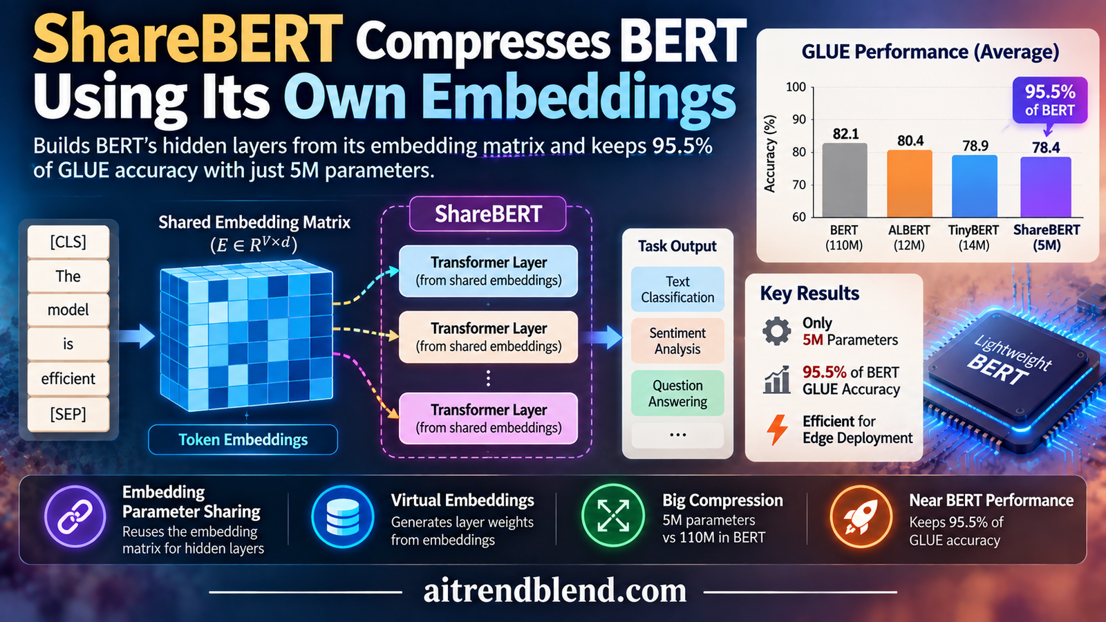
- The Small variant scores 77.8 on the GLUE development average against 81.4 for BERT Base. That is 95.5% of the accuracy with 5.0M parameters, which is 21.9× fewer.
- The Large variant matches BERT Base at 81.4 with 27.0M parameters, a 4.0× reduction, and no knowledge distillation is used.
- The saving is in memory and storage. Compute does not shrink on its own, and the Base variant ran slower than BERT in the authors’ own latency test.
- Word similarity and analogy scores improved rather than degraded, and probing suggests the hidden layers still organize linguistic information in a BERT like way.
- The evidence rests on development sets, a short pretraining budget and a single reported seed, so treat the headline numbers as strong but not settled.
Why the embedding matrix became the wall
Compression research on language models has a habit of stopping at roughly the same place. TinyBERT, ALBERT and YOCO BERT all land near 12 million parameters or above, and the authors point out that this is still too heavy for many IoT devices. The reason is not lack of ingenuity. It is that every trick, whether distillation, pruning or architecture search, works by removing redundancy, and redundancy runs out.
There is also a floor that most methods never touch. Any model that reads text needs an embedding matrix with one vector per token. In BERT Base that matrix accounts for 21% of all parameters, and in the smallest GPT-3 model the paper puts the share at 30%. Shrink the encoder aggressively and the embedding table quietly becomes the largest thing left.
So the Modena group reframed the problem. Instead of asking how to trim the encoder further, they ask why the encoder should own any dedicated weights at all. If the embedding matrix already has to exist, its numbers could be read a second way, as the raw material for the attention and Feed Forward layers. You can read the full study through its open access DOI page, and the code sits in the authors’ GitHub repository.
If you are mapping this against other approaches, our overview of model compression methods covers the families the paper compares against.
What earlier work leaves untouched
Knowledge distillation trains a small student to imitate a large teacher, and it is the most popular route. Pruning removes weights that contribute little. Quantization stores the survivors in fewer bits. Neural architecture search lets an optimizer pick a shape that fits a hardware budget. Each of these shrinks the encoder, and each is still useful.
ALBERT is the closest relative to this paper. It shares one encoder layer across every depth, which is why ALBERT Base gets down to 12M parameters. The catch is built into the idea. You always pay for at least one full layer, and the paper says as much when it compares ALBERT with its own Base model. ShareBERT tries to remove that last fixed cost.
This is also not the authors’ first attempt. An earlier conference version, titled ShareBERT and published at AAAI 2024, first explored sharing embedding parameters with hidden layers. The journal article extends it with a more efficient variant, a wider comparison and experiments on translation and image captioning. Readers who want the distillation side of the story can pair this analysis with our piece on knowledge distillation for language models.
How Embeddings Parameter Sharing works
Carving columns out of the embedding matrix
The first method, called Embeddings Parameter Sharing or EPS, is easiest to picture as a spreadsheet. The embedding matrix has one row per token and one column per feature. EPS reserves some of those columns for a second job. Reading the columns from top to bottom gives a long list of numbers, and those numbers are poured into the weight matrices of the encoder.
How many columns each matrix needs depends on its size. A Feed Forward matrix with hidden size H and intermediate size I holds H times I values. Each attention projection holds H squared values. Divide by the number of tokens E, round up, and you know how many columns to reserve.
Cost of each component
$$L_{HI}=L_{IH}=HI,\qquad L_Q=L_K=L_V=L_O=H^2$$Columns reserved for each component
$$G_{HI}=G_{IH}=\left\lceil \frac{L_{HI}}{E}\right\rceil,\qquad G_Q=G_K=G_V=G_O=\left\lceil \frac{L_Q}{E}\right\rceil$$The condition that limits EPS
$$G_{IH}+G_{HI}+G_Q+G_K+G_V+G_O \le H$$That last inequality is the real constraint. The reserved columns must fit inside the embedding width. With a vocabulary above ten thousand tokens this is easy for one layer, and it is why the authors suggest building a single encoder or decoder layer and sharing it across depth. Because of the rounding, a few values in each reserved column go unused and are simply discarded.
The price of asking numbers to do two jobs
Nothing here comes for free. The same numbers now have to represent words and also act as weights, and those two goals pull in different directions. The ablation shows it. BERT Base with EPS and a Feed Forward size of 3072 falls to 77.0 on the GLUE average, a loss of 4.4 points against the 81.4 baseline. On the Word Analogy test the accuracy drops from 9.9% to 3.3%.
One remedy is to make the network wider. The authors build a hidden size of 2048 with an embedding size of 1152, and the average climbs to 80.9 with 43.0M parameters. That is close to BERT Base at about 40% of its size. It is a good result, but it is not small enough for the microcontroller in our opening scene. The obstacle is that EPS cannot ask for more columns than the embedding has.
Virtual embeddings and the trick behind the small models
The second method, Virtual Embeddings Parameter Sharing or VEPS, removes the width limit with a linear projection. The real embedding matrix stays narrow, with size E by F. A learned projection widens it into a virtual matrix of size E by V. The encoder weights are then carved out of the virtual matrix exactly as in EPS. A second projection brings the input token vectors up to width V so they can enter the encoder.
Virtual embedding matrix and input projection
$$M = T\,W_{F1},\qquad X_0 = \mathrm{Embed}(x)\,W_{F2}$$Here T is the real embedding matrix in \(\mathbb{R}^{E\times F}\) and M is the virtual matrix in \(\mathbb{R}^{E\times V}\).
One reading of this, and it is our reading rather than the authors’ wording, is that VEPS behaves like a small hypernetwork. A compact set of learned numbers, the embedding table and two projections, generates a much larger set of effective weights. That explains a result that looks strange at first. ShareBERT uses a hidden size of 2048, nearly three times BERT Base, and yet the total stays at 5.0M parameters for the Small model.
The three published variants differ mainly in the embedding width. Small uses F equal to 128 with 12 layers. Base uses F equal to 384 with 12 layers. Large uses F equal to 768 with 6 layers. All three share one attention layer and one Feed Forward layer, use V equal to 2048 and an intermediate size of 4096, and work with a 30528 token vocabulary. The Small model has only 1.0M parameters outside its embeddings.
EPS reuses the embedding columns directly and hits a width ceiling. VEPS adds two projections so the hidden layers can be far wider than the embedding, and that single change is what makes 5M parameters possible.
What the numbers say
The table below collects the paper’s ablation rows on the GLUE development set. Read it from the top and the story is clear. Ordinary BERT models that are small enough to compete on size lose several points. Sharing alone recovers some of the gap, and VEPS is the version that gets both size and score.
| Model | Parameters | Compression | GLUE average |
|---|---|---|---|
| BERT Base | 109.5M | 1.0× | 81.4 |
| BERT with hidden size 256 | 17.4M | 6.3× | 77.5 |
| BERT with hidden size 128 | 6.3M | 17.3× | 73.8 |
| BERT plus EPS | 24.5M | 4.4× | 77.0 |
| BERT plus EPS and embedding factorization | 43.0M | 2.5× | 80.9 |
| ShareBERT Small | 5.0M | 21.9× | 77.8 |
| ShareBERT Base | 13.8M | 7.9× | 79.3 |
| ShareBERT Large | 27.0M | 4.0× | 81.4 |
The cleanest comparison is the pair of ShareBERT Small and a plain BERT with hidden size 256. The plain model needs 17.4M parameters to reach 77.5. ShareBERT Small reaches 77.8 with 5.0M. The paper adds that a regular BERT needs up to four times more parameters to match ShareBERT at similar quality.
Against the wider literature, the authors report each method’s relative accuracy against BERT Base, using whatever benchmark subset each original paper used. TinyBERT at 14.5M parameters keeps 96.8% with distillation and 88.8% without it. ShareBERT Small keeps 95.5% with no distillation and about a third of the parameters. That is 1.3 points below distilled TinyBERT and 6.7 points above the undistilled version. ALBERT Base retains 97.3% at 12M, though on a different mix of benchmarks. MicroBERT and KroneckerBERT sit at 98.4% and 97.7% near 14M.
Those comparisons deserve some caution. Some entries use GLUE test sets and others use development sets, and the benchmark subsets differ, which the table footnotes admit. The paper’s text calls the TinyBERT model TinyBERT4 while the table labels it TinyBERT3. The direction of the result is believable, but the exact gaps are soft.
Does sharing hurt what the embeddings learn
A skeptic would worry that loading embeddings with a second job spoils them. The authors test this on word similarity and word analogy, two standard checks on what an embedding table knows.
| Model | Similarity average | Word Analogy | GLUE average |
|---|---|---|---|
| BERT Base | 0.485 | 9.9% | 81.4 |
| BERT plus EPS | 0.264 | 3.3% | 77.0 |
| BERT plus EPS and embedding factorization | 0.506 | 1.9% | 80.9 |
| ShareBERT Small | 0.594 | 10.7% | 77.8 |
| ShareBERT Base | 0.602 | 12.6% | 79.3 |
| ShareBERT Large | 0.638 | 15.2% | 81.4 |
Plain EPS does damage. Analogy accuracy collapses and similarity is mixed, which matches the intuition about competing goals. VEPS reverses the pattern. Every ShareBERT variant beats BERT Base on both measures, and the Large model improves similarity by 0.153 and analogy by 5.3 points.
The authors suggest that involving the embeddings in hidden layer learning gives them access to higher level information about how tokens interact. It is a plausible story, though the paper does not test it directly. Absolute analogy scores are also low for every model, so small differences may say less than the percentages suggest.
A second check uses edge probing, a method that trains tiny classifiers on frozen representations to see where linguistic information lives. In BERT, spelling and syntax show up in early layers while entities, coreference and relations need deeper ones. The authors compare that depth profile between BERT and each ShareBERT variant and report rank correlations of 0.77, 0.77, 0.94, 0.88 and 0.88 across the five comparison models. With access to embeddings only, ShareBERT probes score higher or about equal to BERT on every task. With all twelve layers available there is a slight reduction. The hidden layers seem to still do what BERT layers do, just built from different material.
“Our method reduces the number of initialization options.” Hu, Cavicchioli and Capotondi, Neural Networks 2025, from the limitations section
Shrinking further with ShareBERT Light
The first three variants were designed to prove a point, not to run on a device. Their 2048 wide, 12 layer shape is generous on purpose. The authors then ask how much of that is needed, and the answer is surprisingly little.
Dropping the virtual hidden size from 2048 to 1024 while keeping 12 layers raises the GLUE average to 79.9, above the Base score of 79.3. Going down to 768 gives 79.7. Only when V falls to 384, which equals the embedding width, does the score sag to 77.5. Depth behaves similarly. Six layers score 79.3 and four layers score 78.9, and two layers drop to 76.6. Since none of these choices change the parameter count, the authors settle on V equal to 1024 and four layers.
ShareBERT Light Base has 13.8M parameters and reaches 78.9, or 96.9% of BERT Base. In the paper’s FLOP table it needs 8.85 billion operations against 22.34 billion for BERT. ShareBERT Light Small has 5.0M parameters and scores 77.2, or 94.8%, at 5.83 billion operations.
A small warning about the write up. The text states that both Light models give a 3.83× speedup, and it lists a slightly different configuration for Light Small than Table 4 does. In the table, 3.83× belongs to Light Small alone and Light Base is 2.52×. We used the table figures. The mismatch is minor, but it is the kind of thing you want to check in the released code before designing hardware around it.
Memory is not the same as speed
Where the saving really lands
This is the most important practical point in the paper, and the authors are refreshingly direct about it. Their own measurements on an NVIDIA GeForce RTX 4090 use a batch of 128 sequences of 128 tokens.
| Model | GLUE average | Model memory (MB) | Peak memory (MB) | Time |
|---|---|---|---|---|
| BERT Base | 81.4 | 439 | 745 | 26.7 ms |
| ShareBERT Large | 81.4 | 125 | 845 | 45.8 ms |
| ShareBERT Base | 79.3 | 72 | 792 | 91 ms |
| ShareBERT Small | 77.8 | 36 | 756 | 91 ms |
| ShareBERT Light Base | 78.9 | 52 | 413 | 9 ms |
| ShareBERT Light Small | 77.2 | 19 | 379 | 8.9 ms |
Two things stand out. First, the allocation cost drops by as much as 23 times, from 439 MB to 19 MB. Second, peak memory during a large batch barely moves for the wide variants. ShareBERT Small peaks at 756 MB against 745 MB for BERT, because activations at width 2048 dominate once the weights are small. Latency is worse for the wide models, at 91 ms against 26.7 ms, and better for the Light models at about 9 ms.
The reason is simple. Sharing removes stored parameters but not arithmetic. A 2048 wide layer applied twelve times costs what it costs. Also, the generated weights still have to exist somewhere when the layer runs. The authors note that a suitable low memory inference algorithm would make the reduction useful in practice. Nobody has shown that algorithm here, and this is the gap between a paper result and a shipping product.
Choose the Light configuration when you care about speed and the wide configuration only when you care about the smallest stored file. Judge any deployment by peak memory and latency on your target chip, not by the parameter count alone.
Playing well with quantization and distillation
Because ShareBERT attacks parameter count and not arithmetic, other methods can still be stacked on top. The authors test two. Eight bit quantization applied to the virtual embedding matrix halves the footprint, from 36 MB to 18 MB for Small and from 72 MB to 36 MB for Base. Average accuracy moves by at most 0.1%, so the loss is negligible.
For distillation, they train ShareBERT Light Base as a student with BERT Base as the teacher and a logits matching loss. The GLUE average rises from 78.9 to 80.2, or 98.5% of the teacher. A four layer BERT with 28.7M parameters gains about the same amount, from 79.3 to 80.2. So the method neither blocks distillation nor gets special help from it.
Beyond BERT, translation and image captioning
To show the idea is not tied to Transformers, the authors apply EPS and VEPS to fully attentive, LSTM and convolutional sequence models. The tasks are English to Vietnamese translation on the IWSLT15 set and captioning on the COCO dataset.
| Task and architecture | Without sharing | With VEPS | Compression |
|---|---|---|---|
| Captioning, fully attentive (CIDEr) | 38.6M, 132.8 | 10.2M, 129.5 | 3.78× |
| Captioning, Conv2Seq (CIDEr) | 41.0M, 133.4 | 29.1M, 132.1 | 1.40× |
| Translation, fully attentive (BLEU) | 62.6M, 31.13 | 16.6M, 29.71 | 3.77× |
| Translation, LSTM (BLEU) | 75.3M, 29.01 | 19.8M, 29.34 | 3.80× |
| Translation, Conv2Seq (BLEU) | 81.5M, 27.13 | 48.1M, 29.35 | 1.69× |
Compression here runs from roughly 1.2× to 3.8×, far below the BERT numbers. The paper explains why. The ratio depends on how many modules are shared across depth and how large the embedding matrix is compared with everything else. Even so, at least 95% of baseline quality is retained across the experiments. In translation, VEPS on the convolutional model actually beat its baseline, 29.35 BLEU against 27.13, and the authors even record one case where plain EPS gave a poor initialization in captioning that VEPS avoided.
Where the evidence is thin
The paper is honest about its main limit. EPS and VEPS reduce parameters and were not designed to reduce computation. Beyond that, a careful reader should hold a few reservations.
- The training recipe lists a single seed of 42, and the tables report no variance. RTE scores range from 44.6 to 61.7 across the ablation rows, which suggests that small gaps on that task are noise.
- Pretraining uses 23000 steps on BookCorpus and English Wikipedia with sequences truncated to 128 tokens. That is a modest budget. The BERT baseline is the authors’ own reproduction under the same recipe, so the relative numbers are fair within the paper but not directly comparable to published BERT results.
- Results come from development sets, and the cross paper comparison in Table 1 mixes benchmark subsets and test or development splits.
- Everything runs on a 30528 token English vocabulary. Whether the method holds up with a large multilingual vocabulary, or at the scale of billions of parameters, is untested.
- The method ties initialization of the encoder to the embeddings, which removes some design freedom. The authors argue the effect is small, though it is an open question.
The ideas are sound and the ablations are thorough. What is missing is repeated runs, a bigger pretraining budget and a real device measurement of a low memory inference path.
What this changes for practitioners
If your constraint is flash or model download size, ShareBERT Small is a serious option at 5.0M parameters and 95.5% of the baseline score. If your constraint is latency, start from the Light configuration and measure. If you already distill or quantize, nothing in the paper says you must choose. And if you work on very large vocabularies, the extra columns give the method more room, so it may be worth a small experiment.
The related question of how sharing interacts with transformer attention design is worth a look in our coverage of efficient transformer architectures, and quantization tradeoffs are covered in our guide to post training quantization.
Conclusion
The core achievement is easy to state. ShareBERT shows that a language model can reach 95.5% of BERT Base accuracy on GLUE with 5.0M parameters, and that a 27.0M parameter version matches BERT Base outright. It gets there without knowledge distillation, which means the result comes from the architecture and not from borrowed supervision.
The conceptual shift matters more than any single row of the tables. For years the embedding matrix was treated as fixed overhead, the part of a model you could not touch. This paper treats it as a reservoir of parameters that can be read twice. Once that door opens, the parameter count of an encoder stops being tied to the number of weights the encoder needs.
The idea also travels. The authors apply it to LSTM and convolutional models, to translation and to captioning, and the gains vary but do not vanish. Any system with a large token table and a stack of dense layers is a candidate, including decoder models and multimodal captioners.
The limits are real. Arithmetic is unchanged, wide variants are slower than BERT in the reported test, peak memory does not fall for them, and the results lean on a single seed and a short pretraining run. A practical deployment still needs an inference path that avoids storing the generated weights in full.
The next steps are clear. Test the method with multilingual vocabularies and larger models, measure it on real microcontroller class hardware, and combine it more deeply with quantization and distillation, as the authors themselves propose. If those experiments go well, the floor for useful language models will sit a lot lower than it does today.
Reference implementation in PyTorch
The code below is our own reconstruction of the VEPS model from the paper’s description. It is not the authors’ release, which lives in their repository. Position embeddings, the masked language modeling head, weight tying and the exact column filling order are our assumptions, and the comments say where. We could not execute it in our environment, so treat the smoke test as a starting point and run it before relying on it.
"""
ShareBERT reference sketch (VEPS variant), written from the paper's description.
This is an independent reconstruction, not the authors' released code.
"""
import math
import torch
import torch.nn as nn
import torch.nn.functional as F


# ---------------------------------------------------------------------------
# 1. Column allocator. Decides which columns of the virtual embedding matrix
#    feed which weight matrix, following G = ceil(L / E) from Eq. 3 of the paper.
# ---------------------------------------------------------------------------
class ColumnAllocator:
    def __init__(self, num_tokens, virtual_dim, shapes):
        self.num_tokens = num_tokens
        self.slices = {}
        start = 0
        for name, (rows, cols) in shapes.items():
            cost = rows * cols                        # L for this element
            groups = math.ceil(cost / num_tokens)     # G for this element
            self.slices[name] = (start, groups, rows, cols)
            start += groups
        # Eq. 4 of the paper, the shared groups must fit inside V columns.
        assert start <= virtual_dim, (
            "Need %d columns but the virtual matrix only has %d" % (start, virtual_dim)
        )
        self.total_columns = start

    def build(self, virtual, name):
        start, groups, rows, cols = self.slices[name]
        block = virtual[:, start:start + groups]      # E x G
        flat = block.t().reshape(-1)                  # column by column, top to bottom
        return flat[: rows * cols].reshape(rows, cols)  # unused tail is discarded


# ---------------------------------------------------------------------------
# 2. One shared encoder layer whose dense weights are generated, not stored.
#    Only biases and LayerNorm parameters are learned directly.
# ---------------------------------------------------------------------------
class SharedEncoderLayer(nn.Module):
    def __init__(self, num_tokens, hidden, inter, heads, dropout=0.1):
        super().__init__()
        assert hidden % heads == 0
        self.hidden, self.inter, self.heads = hidden, inter, heads
        shapes = {
            "q": (hidden, hidden), "k": (hidden, hidden),
            "v": (hidden, hidden), "o": (hidden, hidden),
            "hi": (hidden, inter), "ih": (inter, hidden),
        }
        self.allocator = ColumnAllocator(num_tokens, hidden, shapes)
        self.bias_q = nn.Parameter(torch.zeros(hidden))
        self.bias_k = nn.Parameter(torch.zeros(hidden))
        self.bias_v = nn.Parameter(torch.zeros(hidden))
        self.bias_o = nn.Parameter(torch.zeros(hidden))
        self.bias_hi = nn.Parameter(torch.zeros(inter))
        self.bias_ih = nn.Parameter(torch.zeros(hidden))
        self.norm_sa = nn.LayerNorm(hidden)
        self.norm_ff = nn.LayerNorm(hidden)
        self.drop = nn.Dropout(dropout)

    def materialize(self, virtual):
        """Turn the virtual embedding matrix into dense weights, once per forward pass."""
        return {name: self.allocator.build(virtual, name) for name in self.allocator.slices}

    def forward(self, x, w, attend_mask=None):
        b, t, _ = x.shape
        split = lambda z: z.view(b, t, self.heads, -1).transpose(1, 2)
        q = split(x @ w["q"] + self.bias_q)
        k = split(x @ w["k"] + self.bias_k)
        v = split(x @ w["v"] + self.bias_v)
        ctx = F.scaled_dot_product_attention(q, k, v, attn_mask=attend_mask)
        ctx = ctx.transpose(1, 2).reshape(b, t, self.hidden)
        x = self.norm_sa(x + self.drop(ctx @ w["o"] + self.bias_o))
        ff = F.gelu(x @ w["hi"] + self.bias_hi) @ w["ih"] + self.bias_ih
        return self.norm_ff(x + self.drop(ff))


# ---------------------------------------------------------------------------
# 3. The full model. Sizes follow the paper's Small variant by default.
#    Position embeddings, the MLM head and the weight tying are our assumptions.
# ---------------------------------------------------------------------------
class ShareBERT(nn.Module):
    def __init__(self, vocab=30528, emb=128, hidden=2048, inter=4096,
                 layers=12, heads=8, max_len=128, dropout=0.1):
        super().__init__()
        self.layers = layers
        self.tok = nn.Embedding(vocab, emb)          # real embedding matrix, E x F
        self.pos = nn.Embedding(max_len, emb)
        self.w_f1 = nn.Linear(emb, hidden, bias=False)  # builds the virtual matrix, E x V
        self.w_f2 = nn.Linear(emb, hidden)              # conforms inputs to width V
        self.embed_norm = nn.LayerNorm(hidden)
        self.drop = nn.Dropout(dropout)
        self.layer = SharedEncoderLayer(vocab, hidden, inter, heads, dropout)
        # MLM head projects back to F so the output layer can reuse the embeddings.
        self.head_dense = nn.Linear(hidden, emb)
        self.head_norm = nn.LayerNorm(emb)
        self.head_bias = nn.Parameter(torch.zeros(vocab))

    def encode(self, input_ids, attention_mask=None):
        b, t = input_ids.shape
        positions = torch.arange(t, device=input_ids.device).unsqueeze(0)
        x = self.tok(input_ids) + self.pos(positions)
        x = self.drop(self.embed_norm(self.w_f2(x)))
        virtual = self.w_f1(self.tok.weight)            # E x V, shared with the layers
        weights = self.layer.materialize(virtual)
        mask = None
        if attention_mask is not None:
            mask = attention_mask[:, None, None, :].bool()   # True means attend
        for _ in range(self.layers):                    # same weights at every depth
            x = self.layer(x, weights, mask)
        return x

    def mlm_logits(self, hidden_states):
        h = self.head_norm(F.gelu(self.head_dense(hidden_states)))
        return h @ self.tok.weight.t() + self.head_bias

    def forward(self, input_ids, attention_mask=None):
        return self.mlm_logits(self.encode(input_ids, attention_mask))


class Pooler(nn.Module):
    """Used only when fine tuning, as in Fig. 3 of the paper."""
    def __init__(self, hidden, num_classes):
        super().__init__()
        self.dense = nn.Linear(hidden, hidden)
        self.out = nn.Linear(hidden, num_classes)

    def forward(self, hidden_states):
        return self.out(torch.tanh(self.dense(hidden_states[:, 0])))


# ---------------------------------------------------------------------------
# 4. Masked language modeling loss and the usual 80/10/10 corruption.
# ---------------------------------------------------------------------------
def mask_tokens(input_ids, mask_id, vocab, prob=0.15):
    labels = input_ids.clone()
    chosen = torch.rand(input_ids.shape, device=input_ids.device) < prob
    labels[~chosen] = -100
    corrupted = input_ids.clone()
    roll = torch.rand(input_ids.shape, device=input_ids.device)
    corrupted[chosen & (roll < 0.8)] = mask_id
    swap = chosen & (roll >= 0.8) & (roll < 0.9)
    corrupted[swap] = torch.randint(vocab, input_ids.shape, device=input_ids.device)[swap]
    return corrupted, labels


def mlm_loss(logits, labels):
    return F.cross_entropy(logits.view(-1, logits.size(-1)), labels.view(-1), ignore_index=-100)


# ---------------------------------------------------------------------------
# 5. Training loop. Adam with betas 0.9 and 0.98, gradient clipping at 0.5,
#    peak rate 1e-3, linear warmup then linear decay (our reading of Eq. 7).
# ---------------------------------------------------------------------------
def train(model, batches, steps, warmup, mask_id, vocab, peak_lr=1e-3, device="cpu"):
    model.to(device).train()
    opt = torch.optim.Adam(model.parameters(), lr=peak_lr, betas=(0.9, 0.98))
    sched = torch.optim.lr_scheduler.LambdaLR(
        opt,
        lambda s: min((s + 1) / max(1, warmup), max(0.0, (steps - s) / max(1, steps - warmup))),
    )
    history = []
    for step, ids in zip(range(steps), batches):
        ids = ids.to(device)
        corrupted, labels = mask_tokens(ids, mask_id, vocab)
        loss = mlm_loss(model(corrupted), labels)
        opt.zero_grad()
        loss.backward()
        torch.nn.utils.clip_grad_norm_(model.parameters(), 0.5)
        opt.step()
        sched.step()
        history.append(loss.item())
    return history


# ---------------------------------------------------------------------------
# 6. Evaluation. Masked token accuracy and loss on held out batches.
# ---------------------------------------------------------------------------
@torch.no_grad()
def evaluate(model, batches, mask_id, vocab, device="cpu"):
    model.to(device).eval()
    total_loss, correct, seen = 0.0, 0, 0
    for ids in batches:
        ids = ids.to(device)
        corrupted, labels = mask_tokens(ids, mask_id, vocab)
        logits = model(corrupted)
        total_loss += mlm_loss(logits, labels).item()
        keep = labels != -100
        correct += (logits.argmax(-1)[keep] == labels[keep]).sum().item()
        seen += keep.sum().item()
    return {"loss": total_loss / max(1, len(batches)), "masked_acc": correct / max(1, seen)}


def count_parameters(model):
    return sum(p.numel() for p in model.parameters())


# ---------------------------------------------------------------------------
# 7. Smoke test on dummy data. The vocabulary must satisfy E >= 2I + 4V
#    or the allocator will refuse to build the layer.
# ---------------------------------------------------------------------------
if __name__ == "__main__":
    torch.manual_seed(42)
    vocab, mask_id = 1200, 3
    model = ShareBERT(vocab=vocab, emb=32, hidden=128, inter=256,
                      layers=2, heads=4, max_len=32)
    print("parameters", count_parameters(model))
    data = [torch.randint(5, vocab, (8, 32)) for _ in range(20)]
    history = train(model, data, steps=20, warmup=5, mask_id=mask_id, vocab=vocab)
    print("first loss %.3f, last loss %.3f" % (history[0], history[-1]))
    print(evaluate(model, data[:4], mask_id, vocab))
    pooled = Pooler(128, 2)(model.encode(data[0]))
    print("pooler output", tuple(pooled.shape))
Frequently asked questions
What is ShareBERT in plain terms
ShareBERT is a family of BERT style language models whose attention and Feed Forward weights are generated from the embedding matrix instead of being stored on their own. The Small version keeps 95.5% of BERT Base accuracy on GLUE with 5.0M parameters, which is 21.9 times fewer than BERT Base.
How is this different from ALBERT
ALBERT shares one encoder layer across every depth but that layer still needs its own dedicated weights, so there is a fixed cost of at least one full layer. ShareBERT removes that cost by building the layer out of the embedding matrix through Embeddings Parameter Sharing or its virtual variant.
Does ShareBERT run faster than BERT
Not automatically. The paper reports that the wide ShareBERT variants are two to three times slower than BERT Base on an RTX 4090 because arithmetic cost is not reduced by parameter sharing. The Light variants, which use a smaller virtual hidden size and fewer layers, are close to three times faster.
Does sharing embeddings with hidden layers hurt word representations
Plain Embeddings Parameter Sharing does hurt them, cutting Word Analogy accuracy from 9.9% to as low as 3.3% in the paper’s ablation. The Virtual Embeddings variant used in ShareBERT reverses this. Every ShareBERT variant scores higher than BERT Base on the word similarity and word analogy tests reported in the paper.
Can ShareBERT be combined with quantization or knowledge distillation
Yes. The authors apply 8 bit quantization to the virtual embedding matrix with accuracy loss of at most 0.1%, and they train a ShareBERT Light Base student with a BERT Base teacher, raising the GLUE average from 78.9 to 80.2.
Does the method only work on Transformers
No. The paper applies Embeddings Parameter Sharing and its virtual variant to LSTM and convolutional sequence to sequence models as well, testing them on English to Vietnamese translation and image captioning, with at least 95% of baseline quality preserved across the reported configurations.
Hu, J. C., Cavicchioli, R., & Capotondi, A. (2025). Embeddings hidden layers learning for neural network compression. Neural Networks, 191, 107794. https://doi.org/10.1016/j.neunet.2025.107794
This analysis is based on the published paper and an independent evaluation of its claims.