
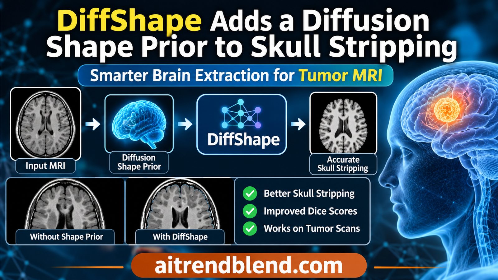
A patient with a newly diagnosed glioblastoma has a T1 weighted MRI before surgery. Before anyone measures the tumor, registers the scan to an atlas or runs a segmentation model, software has to remove everything that is not brain. Skull, scalp, eyes and fat all go. This step, skull stripping, is so routine that it rarely gets a second look. Yet a large tumor pushing against the brain’s edge, or a scan from an unfamiliar scanner, can make it cut away real tissue or leak into the skull, and every later measurement inherits the mistake.
A team from the University of Bath, Fudan University and the University of Cambridge argues that skull stripping networks fail in these cases because they only read pixel intensities. Their method, DiffShape, gives any segmentation network a second input, a brain outline drawn by a diffusion model. The headline gains are real. The more interesting questions are which networks need the help, how much a simple template would have done, and what the diffusion part actually buys.
Key points
- DiffShape describes the outer brain surface as 4096 radii measured from the center of the scan, trains a conditional diffusion model to generate that list from the MRI, and turns the samples into a signed distance map that any network can take as an extra input channel.
- Added to four backbones trained on the CC359 dataset, the prior raised average Dice across three test cohorts by 1.04 to 7.28 points. The largest gains came on GBM125, a glioblastoma cohort the models never saw, by as much as 15.09 points.
- The gains track how badly a backbone fails without help. SegMamba jumped from 77.61 to 92.70 Dice on GBM125, while the in domain CC359 scores barely moved.
- On the glioblastoma scans, only two of the four enhanced backbones beat SynthStrip, an off the shelf tool that was never trained on CC359, and they win by about a quarter of a Dice point.
- A fixed brain template accounts for roughly 40 percent of the 3D U-Net’s average Dice gain by our arithmetic, and a deterministic regression head predicts the shape better in domain, and nearly as well on healthy external scans, for about one fiftieth of the compute per sample.
- Everything was tested on adult T1 weighted scans with simple translation alignment. A 10 degree head rotation degraded the shape prior more than masking out most of a tumor scan.
Medical disclaimer. This article explains published research on brain MRI processing. It is not medical advice, diagnosis or treatment, and it does not evaluate any approved clinical product. Software used on patient scans must be validated and supervised by qualified professionals. If you have questions about your own imaging, please talk to your care team.
Why skull stripping still breaks
Skull stripping, also called brain extraction, separates brain tissue from everything else in a head MRI. It sits at the start of almost every neuroimaging pipeline, from brain volume measurements in dementia research to tumor segmentation and surgical planning. Doing it by hand takes a trained person a long time per scan and different experts draw the edge differently, so automation has been a research target for decades.
The classical tools lean on intensity and simple geometry. BET, the Brain Extraction Tool from Stephen Smith at Oxford, grows a deformable sphere outward until it meets the brain edge. ROBEX from Iglesias and colleagues combines a learned boundary model with a statistical shape model. Both work well on the scans they were tuned for and both need care when protocols change.
Deep learning changed the accuracy picture. Networks like 3D U-Net, nnU-Net from Isensee and colleagues, the transformer based nnFormer and the state space model SegMamba reach Dice scores near 99 percent on data like their training set. SynthStrip from Hoopes and colleagues took a different route and trained on synthetic images with wildly varied contrast, so that it would work on any brain scan without retraining. Foundation models have entered too, and our explainer on adapting the Segment Anything Model to medical images covers the family that two of the paper’s baselines come from.
The authors’ complaint is that all of these deep models learn the brain’s shape only implicitly, as a side effect of predicting a label for each voxel. When the intensities change, through a different scanner, a different protocol or a lesion that looks like skull or fluid, the network has no separate notion of what a brain should look like to fall back on.
“none of these strategies explicitly model global anatomical shape”
Li and colleagues, on augmentation, transformers, state space models and ensembles for skull stripping
Shape priors before DiffShape
Giving a segmenter knowledge of shape is an old idea. Atlas methods register a template brain to the scan and carry its mask across, which works until a tumor or resection makes the registration fail. Statistical shape models capture typical variation with principal components. Learning methods have encoded shape as a signed distance map, where each voxel stores its distance to the surface with a sign for inside or outside, an idea that runs through DeepSDF from Park and colleagues and through medical work that predicts distance maps for organs. Our article on training free deformable registration with FlexiMIND shows how much atlas style methods depend on getting registration right.
Diffusion models add a different tool. A diffusion model learns to turn random noise into realistic samples by reversing a gradual noising process, as introduced in denoising diffusion probabilistic models by Ho, Jain and Abbeel. In medical imaging they have been used for anomaly detection by Wolleb and colleagues, for synthesis and for segmentation. Our article on a treatment aware diffusion model for glioma growth shows the kind of brain tumor MRI work these models now support. The obstacle in 3D is cost. The paper cites reports of full resolution 3D diffusion needing about 80 GB of GPU memory, which pushed earlier work toward 2D slices, patches or compressed latent spaces.
How DiffShape works
DiffShape comes from Yifan Li, Zizheng Li, Haoyu Wang, Yuchen Lu, Carola-Bibiane Schönlieb, Chao Li and Xi Chen, at the University of Bath, Fudan University and the Shanghai Academy of AI for Science, and the University of Cambridge’s Department of Applied Mathematics and Theoretical Physics and Division of Neurosurgery. It is published open access in IEEE Transactions on Medical Imaging, volume 45, issue 10. The trick that makes 3D diffusion affordable is to stop diffusing voxels at all.
A brain as a list of radii
Picture standing at the center of the scan and looking outward in every direction. Along each line of sight, note how far away the brain surface is. If the brain is roughly star convex, meaning every surface point can be seen from the center without the surface folding back in front of it, that set of distances describes the whole outer envelope. The paper argues that this holds well enough for the outer brain boundary, the same assumption that BET’s expanding sphere has made for over two decades.
In practice the authors extract a triangle mesh from the ground truth mask with marching cubes, convert each vertex to spherical coordinates, and split the polar and azimuthal angles into B equal intervals each. That gives B times B bins. In each bin they keep the largest radius, the outermost surface point in that direction, and fill empty bins with the mean of their neighbors. Reading the bins row by row produces one long vector.
Angular bins and the representative radius
$$ \Theta_m = \Big[\tfrac{(m-1)\pi}{B}, \tfrac{m\pi}{B}\Big), \qquad \Phi_n = \Big[\tfrac{(n-1)2\pi}{B}, \tfrac{n\,2\pi}{B}\Big), \qquad m, n \in \{1, \dots, B\} $$ $$ \mathcal{R}_{m,n} = \{\, r_i \mid \theta_i \in \Theta_m,\ \phi_i \in \Phi_n \,\}, \qquad r_j = \max_{r \in \mathcal{R}_{m,n}} r, \quad j = (m-1)B + n $$With \(B = 64\) the brain becomes a vector \(\mathbf{r} \in \mathbb{R}^{4096}\). Empty bins, 4.42 percent of them at this resolution, take the mean of their filled neighbors.
Four thousand numbers instead of a volume of 192 cubed voxels, about seven million, is the whole point. Noise can be added to and removed from a vector this size at negligible cost. The bins are also ordered, so neighboring entries describe neighboring parts of the surface, which a transformer can exploit.
Diffusion over the radii, steered by the image
The forward process adds Gaussian noise to the radius vector step by step until nothing of the brain remains. A network then learns to predict that noise, given the noisy vector, the step number and the MRI itself. The image enters only as a condition. A stack of 3D convolutions encodes the scan, and cross attention lets the radius tokens look at those image features while they are being denoised.
Noising in closed form and the training objective
$$ \hat{\mathbf{r}}_t = \sqrt{\bar{\alpha}_t}\,\mathbf{r} + \sqrt{1 – \bar{\alpha}_t}\,\boldsymbol{\varepsilon}, \qquad \boldsymbol{\varepsilon} \sim \mathcal{N}(\mathbf{0}, \mathbf{I}), \qquad \bar{\alpha}_t = \prod_{k=1}^{t} (1 – \beta_k) $$ $$ \mathcal{L}_{diff} = \mathbb{E}_{t, \mathbf{r}, X} \big\lVert \boldsymbol{\varepsilon} – \boldsymbol{\varepsilon}_{\psi}(\hat{\mathbf{r}}_t, t, X) \big\rVert_2^2 $$\(\beta_t\) rises linearly from \(10^{-4}\) to \(2 \times 10^{-2}\) over \(T = 500\) steps. \(X\) is the MRI volume, and \(\boldsymbol{\varepsilon}_\psi\) is the conditional denoiser.
Two training details turned out to matter. Radii differ in scale across directions, so a plain squared error over all bins is dominated by the large ones. The authors normalize each bin’s residual with training set statistics. They also randomly blank a cube of the input image with probability 0.5 and fill it with noise, which forces the model to complete the shape from partial evidence. In their Table IV, normalization lowered the shape error on all three cohorts, and image masking lowered it further on the radius metric while slightly raising the Chamfer distance on NFBS.
At test time the model needs only the MRI. No mesh extraction runs. A DDIM sampler, the fast deterministic sampler of Song, Meng and Ermon, generates 16 radius vectors per scan from 16 different noise draws. Each is a plausible brain surface, and their spread is meant to capture the model’s uncertainty about the shape.
From radii back to a volume
A segmentation network works on voxels, so each sampled vector is turned back into points along the bin directions and then into a signed distance map. Every voxel gets its distance to the nearest surface point, positive outside the brain and negative inside, judged by whether the voxel lies farther from the grid center than that nearest point.
Signed distance for each sample, then mean, variance and confidence
$$ d^{(s)}(x) = \operatorname{sgn}\!\Big( \lVert x – c \rVert_2 – \lVert p^{*(s)} – c \rVert_2 \Big) \min_k \big\lVert x – p_k^{(s)} \big\rVert_2 $$ $$ \mu_{sdt}(x) = \frac{1}{S}\sum_{s=1}^{S} d^{(s)}(x), \qquad \sigma^2_{sdt}(x) = \frac{1}{S}\sum_{s=1}^{S} \big(d^{(s)}(x) – \mu_{sdt}(x)\big)^2 $$ $$ w(x) = \exp\!\Big[ -\,\sigma^2_{sdt}(x) \big/ \tau_w \Big], \qquad \tau_w = \operatorname{median}_x \sigma^2_{sdt}(x) $$\(c\) is the grid center and \(p^{*(s)}\) the nearest point of sample \(s\). Both maps are smoothed with a Gaussian of 1.5 voxels. The mean map \(\mu_{sdt}\) is the prior that the final model uses.
Plugging the prior into any backbone
The last step is deliberately plain. The mean distance map becomes a second input channel next to the MRI. Only the first layer of the segmentation network changes, adding between 0.001 and 0.027 percent to the parameter count across the four backbones tested. The rest of each architecture and its training recipe stay as published. That simplicity is a strength, since the same prior can be dropped into whatever network a lab already runs.
Key takeaway
DiffShape never asks the diffusion model to segment anything. It generates a coarse brain envelope in a 4096 number space, converts it to a distance map, and lets an ordinary segmentation network use that map as a hint. The authors themselves describe the result as a coarse global geometric anchor, with fine boundaries left to the backbone.
How the experiments were set up
All training used CC359, the Calgary Campinas dataset of Souza and colleagues, with 359 healthy adults aged 29 to 80, scanned on GE, Philips and Siemens machines at 1.5 and 3 tesla. It was split 70 to 30 for training and testing, roughly 251 and 108 scans by our arithmetic. Two cohorts served only as external tests. NFBS contributes 125 healthy adults aged 21 to 45, all scanned on one Siemens 3 tesla scanner model. GBM125 contributes preoperative scans of 125 glioblastoma patients aged 18 to 75, from Siemens and GE 3 tesla scanners, collected with ethics approval and consent. All images are T1 weighted at 1 mm resolution.
Preprocessing is minimal on purpose. Volumes are shifted so their centers match, with no rotation, affine or nonlinear registration, then cropped or padded to 192 voxels a side and normalized to zero mean and unit variance. That choice keeps the comparison fair to methods that do not need registration, and it also means the polar radius representation depends on the head sitting roughly upright and centered.
The comparison set is broad. BET and ROBEX represent classical tools. 3D U-Net, EnNet, nnU-Net, nnFormer, SegMamba and SegFormer3D were retrained on the CC359 training split. PPCS, SynthStrip and LifespanStrip were run as released, and SAM-Med3D and MedSAM2 had only their decoders fine tuned on CC359. DiffShape was added to 3D U-Net, EnNet, nnFormer and SegMamba. The diffusion model trained for up to 200 epochs with Adam on three NVIDIA RTX 3090 GPUs at a batch size of six. Results are reported as Dice in percent and the 95th percentile Hausdorff distance, HD95, in millimetres, with Wilcoxon signed rank tests against each base model.
What the numbers show
| Model | CC359 | NFBS125 | GBM125 | Average |
|---|---|---|---|---|
| SynthStrip, released software | 94.62 / 5.53 | 89.68 / 7.52 | 94.47 / 6.25 | 92.92 / 6.43 |
| nnU-Net | 98.97 / 1.14 | 95.62 / 3.25 | 91.66 / 20.50 | 95.42 / 8.30 |
| 3D U-Net | 97.95 / 2.23 | 94.22 / 5.32 | 93.64 / 7.54 | 95.27 / 5.03 |
| 3D U-Net with DiffShape | 98.84 / 1.26 | 95.37 / 3.62 | 94.72 / 5.96 | 96.31 / 3.61 |
| EnNet | 98.75 / 1.34 | 95.25 / 3.83 | 91.54 / 23.96 | 95.18 / 9.71 |
| EnNet with DiffShape | 98.81 / 1.26 | 95.63 / 3.66 | 94.37 / 6.54 | 96.27 / 3.82 |
| nnFormer | 98.98 / 1.13 | 95.66 / 3.18 | 90.57 / 22.69 | 95.07 / 9.00 |
| nnFormer with DiffShape | 98.98 / 1.14 | 95.99 / 2.95 | 94.69 / 7.18 | 96.55 / 3.76 |
| SegMamba | 98.73 / 2.53 | 89.08 / 8.76 | 77.61 / 44.06 | 88.47 / 18.45 |
| SegMamba with DiffShape | 98.95 / 1.17 | 95.61 / 3.31 | 92.70 / 9.98 | 95.75 / 4.82 |
Every enhanced backbone improves on average. Average Dice rises by 1.04 points for 3D U-Net, 1.09 for EnNet, 1.48 for nnFormer and 7.28 for SegMamba, and average HD95 falls by 1.42, 5.89, 5.24 and 13.63 mm. The paper marks almost every change as significant, the exception being nnFormer on CC359, where Dice is unchanged and HD95 is 0.01 mm worse. The best average Dice in the whole table, 96.55, belongs to nnFormer with DiffShape. One small inconsistency is worth knowing. The results text says the prior raises average Dice by up to 5.1 points and cuts HD95 by up to 12.0 mm, while the table’s own averages put SegMamba’s gains at 7.28 points and 13.63 mm. We quote the table.
The pattern across cohorts is the interesting part. On CC359, where the backbones already score near 99, the prior changes Dice by between 0.00 and 0.89 points. On the healthy external NFBS cohort it trims boundary errors for all four. On glioblastoma scans the effect is large, because that is where the backbones fall apart. Without the prior, all four lose between 4.31 and 21.12 Dice points moving from CC359 to GBM125, and three of them see HD95 balloon past 20 mm, a sign of large chunks of tissue missed or skull included. With the prior, none of them falls below 92.70 Dice on GBM125.
The benefit scales with the failure
SegMamba shows this most clearly. It is excellent in domain at 98.73 Dice, then drops to 77.61 on the tumor cohort with an HD95 of 44.06 mm. The prior lifts it to 92.70 and 9.98 mm, a 15.09 point recovery. 3D U-Net, which was already the most robust of the four on GBM125 at 93.64, gains just 1.08 points. Read one way, DiffShape is a powerful safety net. Read another, much of its headline average gain comes from repairing one backbone that generalizes poorly.
The fairest comparison for a practitioner may be SynthStrip. It was never trained on CC359, it runs as downloadable software, and on GBM125 it scores 94.47 Dice and 6.25 mm, better than every base model there. After adding DiffShape, 3D U-Net reaches 94.72 and nnFormer 94.69, ahead of SynthStrip by a quarter of a point or less. EnNet and SegMamba stay behind it. On HD95 only the 3D U-Net version beats SynthStrip’s 6.25 mm. SynthStrip does score far lower on CC359, 94.62 against about 98 to 99 for the retrained models. Our reading is that some of that gap reflects how CC359’s reference masks draw the brain edge rather than outright errors, since a model trained on those masks learns their conventions. The takeaway is not that DiffShape fails. It is that a strong generalist tool sets a high bar on pathological scans, and the prior lets trained backbones match it rather than leave it behind.
Key takeaway
The prior helps most where a network is weakest. It rescues SegMamba on tumor scans by 15 Dice points, gives the already sturdy 3D U-Net about one point, and leaves in domain scores almost unchanged. On the glioblastoma cohort the enhanced networks end up level with SynthStrip, not far beyond it.
How much of the gain needs a learned shape
Table III of the paper answers a question most readers will have. What if you skip the diffusion model and give the network a simpler prior?
| Prior added to 3D U-Net | CC359 | NFBS125 | GBM125 | Average |
|---|---|---|---|---|
| None | 97.95 / 2.23 | 94.22 / 5.32 | 93.64 / 7.54 | 95.27 / 5.03 |
| Total variation smoothness | 98.82 / 1.34 | 94.78 / 4.70 | 92.77 / 11.53 | 95.46 / 5.86 |
| Fixed template distance map | 98.91 / 1.22 | 94.24 / 6.07 | 93.89 / 7.35 | 95.68 / 4.88 |
| DiffShape predicted distance map | 98.84 / 1.26 | 95.37 / 3.62 | 94.72 / 5.96 | 96.31 / 3.61 |
| Predicted map with confidence weighting | 98.81 / 1.37 | 95.17 / 5.23 | 94.32 / 6.60 | 96.10 / 4.40 |
| Ground truth distance map | 99.19 / 1.02 | 96.24 / 3.35 | 96.86 / 3.03 | 97.43 / 2.47 |
Three readings stand out. First, a single fixed template, the same for every patient, already lifts average Dice from 95.27 to 95.68. That is 0.41 of the 1.04 point gain from DiffShape, roughly 40 percent by our arithmetic, and on CC359 the template actually beats the predicted prior. Where the learned prior earns its keep is outside the training data. On NFBS the template makes HD95 worse, 6.07 mm against 5.32, while the predicted prior improves it to 3.62. On GBM125 the predicted prior cuts HD95 to 5.96 mm against 7.35 for the template. Subject specific shape matters most precisely where the anatomy departs from the average.
Second, the confidence map, the part of the design that uses the spread of the 16 samples, did not help consistently, so the final model drops it. That leaves the mean distance map as the only thing passed on. Averaging 16 samples still smooths the prior, but the uncertainty estimate that motivates sampling is not used for segmentation in the reported results. The paper does suggest it as a visual indicator of where segmentation may be unreliable, around folded cortex and tumor margins.
Third, a perfect prior would do much more. Feeding the ground truth distance map gives 97.43 Dice and 2.47 mm, so there is about 1.1 Dice points and 1.1 mm of headroom left between DiffShape’s prior and an ideal one. Better shape prediction, not a different backbone, is where future gains would come from.
What the diffusion part buys
Could a plain network predict the 4096 radii directly, without diffusion? The authors test this with a two by two design that crosses diffusion against deterministic regression and radial coordinates against Cartesian ones. The regression baselines use the same image encoder and replace the diffusion denoiser with a single prediction head. The metric is the Chamfer distance between predicted and true surface points, in millimetres, as more of the input image is masked out or as the head is rotated.
| Cohort and model | Intact | 50% masked | 90% masked | Rotated 10° | Rotated 20° |
|---|---|---|---|---|---|
| CC359, ViT-Radial regression | 5.84 | 13.64 | 21.60 | 17.33 | 17.42 |
| CC359, Diff-Radial (DiffShape) | 7.39 | 13.73 | 11.24 | 11.86 | 12.87 |
| NFBS125, ViT-Radial regression | 9.93 | 17.38 | 23.46 | 13.74 | 14.38 |
| NFBS125, Diff-Radial (DiffShape) | 9.73 | 14.12 | 12.54 | 12.36 | 13.44 |
| GBM125, ViT-Radial regression | 8.23 | 16.29 | 25.65 | 17.36 | 17.68 |
| GBM125, Diff-Radial (DiffShape) | 7.08 | 10.53 | 10.34 | 13.25 | 14.34 |
On intact in domain scans the simpler regression model wins, 5.84 mm against 7.39. On the external cohorts diffusion is ahead, narrowly on NFBS and by about 1.2 mm on GBM125. Under heavy masking the gap becomes dramatic. Hide 90 percent of the brain and the regression model’s error more than doubles, while the diffusion model’s rises by only 3 to 4 mm, because it can fall back on its learned shape distribution. Radial coordinates also beat Cartesian ones in both paradigms on intact scans, which supports the choice of representation.
Rotation is the uncomfortable result. A 10 degree tilt raises the diffusion model’s error on GBM125 from 7.08 to 13.25 mm, worse than its error with 90 percent of the image masked. The authors frame this as diffusion being more robust than regression, which is true, since regression degrades even more. But it also shows that the polar representation, anchored to the grid center and a fixed angular grid, is sensitive to head pose. Patients do not always lie perfectly straight in a scanner, and the paper aligns only by translation.
Two questions are left open. The masking and rotation tests measure the prior’s geometry, not skull stripping accuracy, so we do not know whether a regression prior fed into the same backbones would have given similar Dice. And the cost difference is large. The paper’s Table IX lists the diffusion model at 106.5 million parameters and 37.37 trillion operations for one 50 step sample, against 0.75 for the single pass regression model, about 50 times more. With 16 samples per scan, as Algorithm 2 describes, that is roughly 600 trillion operations per scan by our arithmetic. The paper reports no wall clock inference time for the diffusion model and names faster few step samplers as future work.
“a coarse global geometric anchor”
Li and colleagues, describing the role of the DiffShape distance map
Resolution and other settings
The angular resolution B behaves sensibly. The authors tested 16, 32, 64 and 128 bins per angle. Segmentation quality rises up to B of 64 and slightly drops at 128, which they read as an overly fine prior constraining the backbone too much. When preparing training data, building the radius vector takes about 0.20 seconds per volume at every resolution, 70.8 times faster than casting rays against the mesh at B of 64, and the error from filling empty bins is 1.67 voxels on average.
Two hyperparameter results are worth knowing for anyone reimplementing it. Doubling the number of diffusion steps to 1000 made the radius error about five times larger on CC359, 30.16 against 6.01, which the paper does not explain. And eight samples per scan gave Chamfer distances within 0.2 mm of sixteen on all three cohorts, and slightly better on two of them, so halving the sampling cost appears to lose little.
Clinical translation gap
Skull stripping is rarely the end product. Its output feeds volume measurements, registration and tumor segmentation, so its errors arrive downstream quietly. That makes the gap between these results and clinical use matter, even for a preprocessing step.
The scope is narrow. Every scan is T1 weighted, from adults, at 1 mm resolution. There are no T2, FLAIR or contrast enhanced images, no children or infants, and no postoperative scans, even though the paper’s introduction names resections and implants as the cases that break atlas methods. The glioblastoma cohort is preoperative only. SynthStrip and LifespanStrip were built for exactly the broader range of contrasts and ages that this study does not test.
The evaluation stops at overlap and boundary metrics. There is no reader study, no check of how the masks change tumor volumes or brain volume estimates, and no test of a full pipeline. The confidence map is proposed as an indicator of unreliable regions, but its value for flagging failures to a human was not measured.
Practical constraints also matter. The method assumes heads are centered and roughly upright, and a 10 degree rotation nearly doubled the prior’s error on tumor scans. Inference needs many passes through a 106.5 million parameter model per scan, with no reported running time. And the external tumor cohort, while valuable, is a single collection of 125 patients from two scanner vendors.
Regulatory and safety note, our reading
Brain extraction software used inside a clinical pipeline, such as tumor volumetry or surgical planning, would be part of a regulated medical device in most jurisdictions. A component whose accuracy depends on head orientation and image contrast would need validation on each scanner and protocol it meets, reporting by patient group including postoperative and pediatric cases, automated checks that catch failed masks, and review of outputs by qualified staff before any measurement is used for care.
Limitations, sample size and bias
- One training dataset. All learned models trained on the CC359 split of roughly 251 healthy adults, so the external results show transfer from one healthy population, not from a diverse training mix.
- Small external cohorts. NFBS and GBM125 hold 125 scans each. NFBS comes from a single scanner model and a narrow age range of 21 to 45.
- T1 weighted adults only. No other contrasts, no pediatric or elderly extremes beyond 80, and no postoperative anatomy were tested.
- Pose sensitivity. Alignment is by translation only, and the shape prior degrades sharply with modest rotation, from 7.08 to 13.25 mm Chamfer distance on GBM125 at 10 degrees.
- Star convex assumption. One radius per direction cannot represent surfaces that fold back, which the authors acknowledge limits the method to the outer brain envelope.
- Uneven gains. Most of the average improvement comes from backbones that generalize badly without help, and two of four enhanced models remain behind SynthStrip on the tumor cohort.
- Unanswered ablation. The paper does not test a deterministic regression prior inside the segmentation backbones, so the downstream value of diffusion over a 50 times cheaper alternative is unmeasured. It also does not say whether the backbones were trained with priors predicted on their own training scans or held out predictions, which affects how well training matches test conditions.
- Reporting gaps. The text and Table II disagree on the size of the largest gains, inference time is not reported, and nnU-Net, the strongest base model on average Dice, was not tested with the prior.
What practitioners can take from this
If your skull stripping network works well in domain but falls apart on tumors or new scanners, a shape prior channel is a cheap change to try. The first layer gains one input channel and nothing else changes. Start with a fixed template distance map, since in this paper it delivered about 40 percent of the gain on 3D U-Net at no inference cost. Move to a learned, subject specific prior if your failures cluster on unusual anatomy.
If you adopt DiffShape itself, reorient scans to a standard pose before running it, given the rotation results. Try eight samples instead of sixteen. Keep a strong generalist like SynthStrip in your comparison, especially on pathological data, because the bar it sets is high.
If you are building on the idea, the paper points to clear next experiments. Feed a regression prior into the same backbones to measure what diffusion adds downstream. Test with rotation augmentation and other contrasts. And try representations that handle folded surfaces, since the polar radius trick is specific to the outer brain envelope. Related work on this site approaches brain MRI from other angles. Our article on HGA and unevenly missing MRI sequences deals with brain tumor segmentation when inputs are absent, and our piece on Diffuse2Seg and diffusion based segmentation takes diffusion models in another direction. More studies of this kind sit in our Medical AI section.
Conclusion
DiffShape makes a clean argument and backs it with careful experiments. Skull stripping networks know brain shape only implicitly, so when intensities mislead them they have nothing to fall back on. Giving them an explicit, patient specific shape as an extra input channel improved every one of four very different backbones on average, and it rescued the weakest of them on glioblastoma scans by 15 Dice points.
The conceptual move is to separate what a brain looks like from where its edge is likely to be. By diffusing a list of radii instead of a volume, the authors make 3D generative shape modeling cheap enough to train on ordinary GPUs, and by passing the result as a distance map they keep the segmentation backbone in charge of fine detail. That division of labor is the part most likely to travel.
It could travel well. Any task whose target is a single closed, roughly convex surface, such as the outer outline of certain organs, the skull itself or an implant’s envelope, could use the same polar trick. Tasks with folded or branching structures would need a different compact representation, but the recipe of generating a coarse shape and handing it to an existing network as an extra channel does not depend on the details.
The evidence still has gaps. Training used one healthy adult dataset, the external cohorts are 125 scans each, everything is T1 weighted, and head rotation hurts the prior badly. A fixed template captures a large share of the benefit in domain, a regression head predicts shape nearly as well for a fraction of the compute, and the downstream value of diffusion over regression was not measured. On tumor scans, the enhanced networks reach the level of SynthStrip rather than surpassing it by much.
The next study should test the prior inside backbones against a regression prior and a template, on rotated scans, other contrasts, children and postoperative brains, and report running time alongside accuracy. If the learned prior still wins there, DiffShape will have earned a permanent place at the front of brain MRI pipelines.
Skull stripping is the step everyone assumes works. This paper is a useful reminder that the first cut in a pipeline deserves as much scrutiny as the last.
A reference implementation in PyTorch
The authors release their implementation and pretrained models through their GitHub repository, and that is the version to use for any real comparison. The listing below is our own editorial reconstruction, written so that every equation runs. It builds the polar radius vector from a mask with marching cubes, normalizes radii per bin, trains a conditional denoiser with a 3D convolutional encoder, radius tokens and cross attention, samples with DDIM, converts the samples to signed distance maps with mean, variance and confidence, and trains a small 3D U-Net with and without the prior channel. It also trains a deterministic regression head for the diffusion versus regression check, and evaluates Dice and HD95 on in domain, contrast shifted and lesion bearing synthetic volumes.
We ran the listing on a CPU with 64 synthetic training volumes of 24 voxels a side, each a star convex brain inside a dark fluid gap, a skull and a bright scalp layer. It was tested on 16 volumes with the training contrast, 16 with weaker contrast and a bias field, and 16 more that also carry a dark lesion at the brain edge. One deviation matters. The paper’s noise prediction objective did not learn to use the image within our small CPU budget, and its samples simply matched the mean training shape. The smoke test therefore predicts the clean radius vector instead, which is the same model reparameterized, and the code keeps the paper’s objective as the default option.
The diffusion prior’s surface error was 0.70 to 0.72 voxels on the three test sets, level with the regression head at 0.68 to 0.72, much like the paper’s in domain pattern. Every segmenter scored 100 percent Dice on the training contrast, so the toy is easy there. Under the contrast shift the plain U-Net was unstable. Across three training seeds it scored 91.25, 77.21 and 55.58 Dice, while the same U-Net with the predicted prior scored 92.47, 93.34 and 92.64. On the lesion set the figures were 88.89, 73.33 and 52.79 without the prior and 90.02, 91.11 and 89.72 with it. A ground truth prior reached 96.29 and 93.70 with the first seed. The fixed template prior collapsed to 16.20 and 14.83 in its single run, the opposite of the paper’s finding, which is a reminder that a toy this small says nothing about the paper’s numbers. Treat the listing as a way to read the equations, and use the authors’ repository for anything you would report.
"""
DiffShape reference sketch in PyTorch
=====================================
An editorial reconstruction of DiffShape from Li, Li, Wang, Lu, Schonlieb, Li and Chen,
"DiffShape: Decoupling Shape Priors With Conditional Diffusion for Robust Brain
Extraction", IEEE Transactions on Medical Imaging 45(10), 2026, 5178 to 5190,
DOI 10.1109/TMI.2026.3716658. This is NOT the authors' code. Their implementation and
pretrained models are at github.com/lyf7374/DiffShape.

What is here
  * Algorithm 1: brain mask -> marching cubes mesh -> spherical coordinates around the
    grid centre -> B x B angular bins -> largest radius per bin -> 8 neighbour imputation
    of empty bins -> polar radius vector r of length B^2 (Eqs. 1 to 3).
  * Radius normalisation with per bin training statistics (Table IV of the paper).
  * Forward noising with a linear beta schedule (Eqs. 4 and 5).
  * A conditional denoiser: 3D conv image encoder, radius tokens plus a time embedding,
    self attention and cross attention to the image tokens, trained with the noise
    prediction loss (Eqs. 6 and 7) and random cubic image masking (p = 0.5).
  * DDIM sampling of S posterior shapes per scan (Algorithm 2, phase 3).
  * Polar radius vector -> point cloud -> signed distance map (Eq. 8), voxel wise mean
    and variance over samples (Eqs. 9 and 10), Gaussian smoothing, confidence field (Eq. 11).
  * A small 3D U-Net whose first layer takes the MRI plus the mean SDT prior as two
    channels, compared with the same U-Net on the MRI alone, a fixed template SDT and the
    ground truth SDT (the structure of Table III).
  * A deterministic regression head on the same encoder, for a diffusion versus
    regression check of the prior's Chamfer distance (the idea behind Table VI).
  * Dice and HD95 evaluation on an in domain test set, a contrast shifted set and a set
    with a simulated mass lesion.

Simplifications, stated plainly
  * Synthetic 24^3 star convex "brains" with a skull shell instead of real T1 scans, so the
    script runs on a CPU in a few minutes. Numbers from it say nothing about the paper's.
  * B = 16 (256 bins) instead of 64, 20 DDIM steps instead of 50, S = 8 samples instead
    of 16, and a far smaller network than the paper's 106.5 M parameters. T = 500 and the
    beta range 1e-4 to 2e-2 follow the paper. With a shorter chain the forward process
    never reaches pure noise, which breaks sampling from noise.
  * The paper trains the noise prediction objective of Eq. 7, and train_denoiser does that
    by default. With 64 toy volumes and a CPU budget, that objective did not learn to use the
    image (its samples matched the mean training shape), so the smoke test sets
    objective="x0" and predicts the clean vector instead. This is the same model
    reparameterised, but the loss weighting differs from the paper's.
  * The paper does not say how the SDT channel is scaled before entering the backbone.
    We divide it by 8 voxels. The Chamfer distance here is the mean of the two directed
    nearest neighbour distances, in voxels.
"""
import math
import time

import numpy as np
import torch
import torch.nn as nn
import torch.nn.functional as F
from scipy import ndimage
from skimage.measure import marching_cubes

torch.set_num_threads(2)


# ---------------------------------------------------------------------------
# 1. Polar radius representation (Algorithm 1, Eqs. 1 to 3)
# ---------------------------------------------------------------------------
def grid_centre(shape):
    return np.array([(s - 1) / 2.0 for s in shape], dtype=np.float64)


def mask_to_polar_radius(mask, B):
    """Ground truth polar radius vector of length B*B for one binary mask."""
    verts, _, _, _ = marching_cubes(mask.astype(np.float32), level=0.5)
    v = verts - grid_centre(mask.shape)
    r = np.linalg.norm(v, axis=1)
    theta = np.arccos(np.clip(v[:, 2] / np.maximum(r, 1e-8), -1.0, 1.0))      # [0, pi]
    phi = np.mod(np.arctan2(v[:, 1], v[:, 0]), 2 * np.pi)                      # [0, 2 pi)
    m = np.minimum((theta / np.pi * B).astype(int), B - 1)                     # Eq. 1
    n = np.minimum((phi / (2 * np.pi) * B).astype(int), B - 1)
    grid = np.full((B, B), np.nan)
    for mi, ni, ri in zip(m, n, r):                                            # Eqs. 2 and 3
        if np.isnan(grid[mi, ni]) or ri > grid[mi, ni]:
            grid[mi, ni] = ri
    empty_fraction = float(np.isnan(grid).mean())
    while np.isnan(grid).any():                                                # 8 neighbour mean
        filled = grid.copy()
        for mi, ni in zip(*np.where(np.isnan(grid))):
            nb = [grid[a, b % B] for a in range(mi - 1, mi + 2) for b in range(ni - 1, ni + 2)
                  if 0 <= a < B and not (a == mi and b % B == ni) and not np.isnan(grid[a, b % B])]
            if nb:
                filled[mi, ni] = float(np.mean(nb))
        grid = filled
    return grid.reshape(-1).astype(np.float32), empty_fraction                  # row major


def bin_directions(B):
    """Unit vectors through the centre of each (theta, phi) bin, row major."""
    th = (np.arange(B) + 0.5) * np.pi / B
    ph = (np.arange(B) + 0.5) * 2 * np.pi / B
    T, P = np.meshgrid(th, ph, indexing="ij")
    d = np.stack([np.sin(T) * np.cos(P), np.sin(T) * np.sin(P), np.cos(T)], -1)
    return torch.tensor(d.reshape(-1, 3), dtype=torch.float32)


def polar_to_points(r, dirs, centre):
    """r of shape (..., B*B) -> points (..., B*B, 3) in voxel coordinates."""
    return centre + r.unsqueeze(-1) * dirs


# ---------------------------------------------------------------------------
# 2. Signed distance prior (Eqs. 8 to 11)
# ---------------------------------------------------------------------------
def voxel_coords(shape):
    zz = torch.stack(torch.meshgrid(*[torch.arange(s, dtype=torch.float32) for s in shape],
                                    indexing="ij"), -1)
    return zz.reshape(-1, 3)


def sdt_from_points(points, shape, centre, coords=None):
    """Eq. 8. Negative inside the predicted surface, positive outside."""
    coords = voxel_coords(shape) if coords is None else coords
    dist = torch.cdist(coords, points)                                       # (V, K)
    dmin, idx = dist.min(1)
    p_star = points[idx]
    sign = torch.sign((coords - centre).norm(dim=1) - (p_star - centre).norm(dim=1))
    sign[sign == 0] = 1.0
    return (sign * dmin).reshape(shape)


def shape_prior_from_samples(r_samples, dirs, shape, smooth_sigma=1.5):
    """Eqs. 9 to 11 for S sampled radius vectors of one scan."""
    centre = torch.tensor(grid_centre(shape), dtype=torch.float32)
    coords = voxel_coords(shape)
    sdts = torch.stack([sdt_from_points(polar_to_points(r, dirs, centre), shape, centre, coords)
                        for r in r_samples])
    mu = sdts.mean(0).numpy()                                                 # Eq. 9
    var = sdts.var(0, unbiased=False).numpy()                                 # Eq. 10
    mu = ndimage.gaussian_filter(mu, smooth_sigma)
    var = ndimage.gaussian_filter(var, smooth_sigma)
    tau = max(float(np.median(var)), 1e-6)
    w = np.exp(-var / tau)                                                    # Eq. 11
    return mu.astype(np.float32), w.astype(np.float32)


def chamfer(a, b):
    d = torch.cdist(a, b)
    return 0.5 * (d.min(1).values.mean() + d.min(0).values.mean()).item()


# ---------------------------------------------------------------------------
# 3. Noise schedule (Eqs. 4 and 5) and DDIM sampler
# ---------------------------------------------------------------------------
class LinearSchedule:
    def __init__(self, T=500, beta_start=1e-4, beta_end=2e-2):
        self.T = T
        self.betas = torch.linspace(beta_start, beta_end, T)
        self.abar = torch.cumprod(1.0 - self.betas, 0)

    def q_sample(self, r0, t, eps):
        a = self.abar[t].unsqueeze(-1)
        return a.sqrt() * r0 + (1 - a).sqrt() * eps                           # Eq. 5


@torch.no_grad()
def ddim_sample(model, image, sched, steps=20, n_samples=8, dim=256, objective="eps"):
    """Deterministic DDIM (eta = 0). image is (1, 1, D, H, W). Returns (S, dim).
    objective "eps" means the network predicts the noise (Eq. 6, the paper's choice).
    objective "x0" means it predicts the clean vector, which is the same model
    reparameterised, eps = (r_t - sqrt(abar) x0) / sqrt(1 - abar)."""
    model.eval()
    img = image.expand(n_samples, -1, -1, -1, -1)
    x = torch.randn(n_samples, dim)
    ts = torch.linspace(sched.T - 1, 0, steps).long()
    for i, t in enumerate(ts):
        a_t = sched.abar[t]
        a_prev = sched.abar[ts[i + 1]] if i + 1 < len(ts) else torch.tensor(1.0)
        out = model(x, torch.full((n_samples,), int(t)), img)
        if objective == "eps":
            eps = out
            x0 = (x - (1 - a_t).sqrt() * eps) / a_t.sqrt()
        else:
            x0 = out
            eps = (x - a_t.sqrt() * x0) / (1 - a_t).sqrt()
        x = a_prev.sqrt() * x0 + (1 - a_prev).sqrt() * eps
    return x


# ---------------------------------------------------------------------------
# 4. Conditional denoiser eps_psi(r_t, t, X) (Eq. 6)
# ---------------------------------------------------------------------------
def timestep_embedding(t, dim):
    half = dim // 2
    freqs = torch.exp(-math.log(10000) * torch.arange(half, dtype=torch.float32) / half)
    args = t.float().unsqueeze(1) * freqs.unsqueeze(0)
    return torch.cat([args.sin(), args.cos()], 1)


class ImageEncoder3D(nn.Module):
    """Several strided 3D conv blocks, size^3 -> (size / 8)^3 image tokens."""

    def __init__(self, d=96, n_tokens=27):
        super().__init__()
        def blk(i, o):
            return nn.Sequential(nn.Conv3d(i, o, 3, 2, 1), nn.GroupNorm(4, o), nn.SiLU(),
                                 nn.Conv3d(o, o, 3, 1, 1), nn.GroupNorm(4, o), nn.SiLU())
        self.net = nn.Sequential(blk(1, 16), blk(16, 32), blk(32, 64))
        self.proj = nn.Linear(64, d)
        self.pos = nn.Parameter(torch.zeros(1, n_tokens, d))

    def forward(self, x):
        f = self.net(x).flatten(2).transpose(1, 2)                            # (N, tokens, 64)
        return self.proj(f) + self.pos


class ShapeBlock(nn.Module):
    def __init__(self, d, heads=4):
        super().__init__()
        self.n1, self.n2, self.n3 = nn.LayerNorm(d), nn.LayerNorm(d), nn.LayerNorm(d)
        self.self_attn = nn.MultiheadAttention(d, heads, batch_first=True)
        self.cross_attn = nn.MultiheadAttention(d, heads, batch_first=True)
        self.mlp = nn.Sequential(nn.Linear(d, 4 * d), nn.GELU(), nn.Linear(4 * d, d))

    def forward(self, h, ctx):
        q = self.n1(h)
        h = h + self.self_attn(q, q, q, need_weights=False)[0]
        h = h + self.cross_attn(self.n2(h), ctx, ctx, need_weights=False)[0]   # align shape with image
        return h + self.mlp(self.n3(h))


class ConditionalShapeDenoiser(nn.Module):
    """Predicts the noise on a (normalised) polar radius vector, given t and the MRI."""

    def __init__(self, B=16, d=96, depth=3, n_tokens=27):
        super().__init__()
        self.B, self.d = B, d
        self.enc = ImageEncoder3D(d, n_tokens)
        self.r_in = nn.Linear(B, d)                                           # one token per theta ring
        self.r_pos = nn.Parameter(torch.zeros(1, B, d))
        self.t_mlp = nn.Sequential(nn.Linear(d, d), nn.SiLU(), nn.Linear(d, d))
        self.blocks = nn.ModuleList([ShapeBlock(d) for _ in range(depth)])
        self.out = nn.Sequential(nn.LayerNorm(d), nn.Linear(d, B))

    def forward(self, r_t, t, image):
        ctx = self.enc(image)
        h = self.r_in(r_t.view(-1, self.B, self.B)) + self.r_pos
        h = h + self.t_mlp(timestep_embedding(t, self.d)).unsqueeze(1)
        for blk in self.blocks:
            h = blk(h, ctx)
        return self.out(h).reshape(-1, self.B * self.B)


class RadiusRegressor(nn.Module):
    """Deterministic comparison: same encoder, MLP head straight to r (no diffusion)."""

    def __init__(self, B=16, d=96, n_tokens=27):
        super().__init__()
        self.enc = ImageEncoder3D(d, n_tokens)
        self.head = nn.Sequential(nn.LayerNorm(d), nn.Linear(d, 256), nn.GELU(), nn.Linear(256, B * B))

    def forward(self, image):
        return self.head(self.enc(image).mean(1))


def random_cubic_mask(images, p=0.5, lo=4, hi=10):
    """Training augmentation. Replace a random cube with Gaussian noise."""
    out = images.clone()
    for i in range(out.shape[0]):
        if torch.rand(()) < p:
            s = int(torch.randint(lo, hi + 1, ()))
            z, y, x = [int(torch.randint(0, out.shape[k + 2] - s + 1, ())) for k in range(3)]
            out[i, :, z:z + s, y:y + s, x:x + s] = torch.randn(1, s, s, s)
    return out


def n_image_tokens(images):
    return (images.shape[-1] // 8) ** 3


def train_denoiser(images, r_norm, sched, B=16, epochs=80, bs=16, lr=3e-4, seed=0, objective="eps"):
    torch.manual_seed(seed)
    model = ConditionalShapeDenoiser(B, n_tokens=n_image_tokens(images))
    opt = torch.optim.Adam(model.parameters(), lr=lr)
    n = images.shape[0]
    for ep in range(epochs):
        model.train()
        perm = torch.randperm(n)
        for i in range(0, n, bs):
            idx = perm[i:i + bs]
            x0, img = r_norm[idx], random_cubic_mask(images[idx])
            t = torch.randint(0, sched.T, (len(idx),))
            eps = torch.randn_like(x0)
            target = eps if objective == "eps" else x0
            loss = F.mse_loss(model(sched.q_sample(x0, t, eps), t, img), target)  # Eq. 7 when "eps"
            opt.zero_grad(); loss.backward(); opt.step()
    return model


def train_regressor(images, r_norm, B=16, epochs=80, bs=16, lr=3e-4, seed=0):
    torch.manual_seed(seed)
    model = RadiusRegressor(B, n_tokens=n_image_tokens(images))
    opt = torch.optim.Adam(model.parameters(), lr=lr)
    n = images.shape[0]
    for ep in range(epochs):
        model.train()
        perm = torch.randperm(n)
        for i in range(0, n, bs):
            idx = perm[i:i + bs]
            loss = F.mse_loss(model(random_cubic_mask(images[idx])), r_norm[idx])
            opt.zero_grad(); loss.backward(); opt.step()
    return model


# ---------------------------------------------------------------------------
# 5. Downstream skull stripping backbone with an extra prior channel
# ---------------------------------------------------------------------------
class TinyUNet3D(nn.Module):
    def __init__(self, in_ch=1, c=8):
        super().__init__()
        def cb(i, o):
            return nn.Sequential(nn.Conv3d(i, o, 3, 1, 1), nn.GroupNorm(4, o), nn.SiLU(),
                                 nn.Conv3d(o, o, 3, 1, 1), nn.GroupNorm(4, o), nn.SiLU())
        self.e1, self.e2, self.e3 = cb(in_ch, c), cb(c, 2 * c), cb(2 * c, 4 * c)
        self.u2, self.d2 = nn.ConvTranspose3d(4 * c, 2 * c, 2, 2), cb(4 * c, 2 * c)
        self.u1, self.d1 = nn.ConvTranspose3d(2 * c, c, 2, 2), cb(2 * c, c)
        self.head = nn.Conv3d(c, 1, 1)

    def forward(self, x):
        e1 = self.e1(x)
        e2 = self.e2(F.max_pool3d(e1, 2))
        e3 = self.e3(F.max_pool3d(e2, 2))
        d2 = self.d2(torch.cat([self.u2(e3), e2], 1))
        d1 = self.d1(torch.cat([self.u1(d2), e1], 1))
        return self.head(d1)


def dice_bce(logits, target):
    p = torch.sigmoid(logits)
    inter = (p * target).sum((1, 2, 3, 4))
    dice = 1 - (2 * inter + 1) / (p.sum((1, 2, 3, 4)) + target.sum((1, 2, 3, 4)) + 1)
    return dice.mean() + F.binary_cross_entropy_with_logits(logits, target)


def train_segmenter(inputs, masks, epochs=30, bs=8, lr=2e-3, seed=0):
    torch.manual_seed(seed)
    net = TinyUNet3D(in_ch=inputs.shape[1])
    opt = torch.optim.Adam(net.parameters(), lr=lr)
    n = inputs.shape[0]
    for ep in range(epochs):
        net.train()
        perm = torch.randperm(n)
        for i in range(0, n, bs):
            idx = perm[i:i + bs]
            loss = dice_bce(net(inputs[idx]), masks[idx])
            opt.zero_grad(); loss.backward(); opt.step()
    return net


def hd95(pred, gt):
    if pred.sum() == 0 or gt.sum() == 0:
        return float("nan")
    sp = pred ^ ndimage.binary_erosion(pred)
    sg = gt ^ ndimage.binary_erosion(gt)
    dt_g = ndimage.distance_transform_edt(~sg)
    dt_p = ndimage.distance_transform_edt(~sp)
    return float(np.percentile(np.concatenate([dt_g[sp], dt_p[sg]]), 95))


@torch.no_grad()
def evaluate_segmenter(net, inputs, masks):
    net.eval()
    pred = (torch.sigmoid(net(inputs)) > 0.5).numpy()[:, 0]
    gt = masks.numpy()[:, 0] > 0.5
    dice = [2 * (p & g).sum() / (p.sum() + g.sum() + 1e-8) for p, g in zip(pred, gt)]
    return 100 * float(np.mean(dice)), float(np.nanmean([hd95(p, g) for p, g in zip(pred, gt)]))


# ---------------------------------------------------------------------------
# 6. Synthetic brains, skulls, contrast shift and mass lesions
# ---------------------------------------------------------------------------
def synth_case(rng, size=24, domain="train", lesion=False):
    c = grid_centre((size,) * 3) + rng.uniform(-1.0, 1.0, 3)
    zz, yy, xx = np.meshgrid(*[np.arange(size)] * 3, indexing="ij")
    v = np.stack([xx, yy, zz], -1) - c[::-1]                                  # (x, y, z) offsets
    v = v[..., ::-1]
    r = np.linalg.norm(v, axis=-1) + 1e-8
    th = np.arccos(np.clip(v[..., 2] / r, -1, 1))
    ph = np.arctan2(v[..., 1], v[..., 0])
    R = 0.30 * size + rng.uniform(-0.6, 0.6)
    R = R * (1 + 0.12 * np.cos(th) ** 2 - 0.08 * np.sin(th) ** 2 * np.cos(2 * ph))
    for _ in range(3):                                                        # subject specific folds
        a, k, l, s = rng.uniform(0.02, 0.06), rng.integers(1, 4), rng.integers(1, 4), rng.uniform(0, 6.3)
        R = R * (1 + a * np.sin(k * th + s) * np.cos(l * ph + s))
    if lesion:                                                                # mass effect bulge
        lt, lp = rng.uniform(0.6, 2.4), rng.uniform(-np.pi, np.pi)
        ang = np.arccos(np.clip(np.sin(th) * np.sin(lt) * np.cos(ph - lp) + np.cos(th) * np.cos(lt), -1, 1))
        R = R * (1 + 0.18 * np.exp(-(ang / 0.45) ** 2))
    brain = r <= R
    csf = (r > R) & (r <= R + 0.04 * size)                                     # thin dark gap
    skull = (r > R + 0.04 * size) & (r <= R + 0.10 * size)
    scalp = (r > R + 0.10 * size) & (r <= R + 0.16 * size)                     # bright fat layer
    texture = ndimage.gaussian_filter(rng.normal(0, 1, (size,) * 3), 1.2)
    if domain == "train":                                                     # T1 like contrast
        img = 0.02 + brain * (0.83 + 0.10 * texture) + csf * 0.13 + skull * 0.28 + scalp * 0.78
        noise = 0.04
    else:                                                                     # weaker contrast, bias
        bias = 1 + 0.4 * ((zz - size / 2) / size)
        img = (0.05 + brain * (0.55 + 0.15 * texture) + csf * 0.48 + skull * (0.45 + 0.10 * texture)
               + scalp * 0.95) * bias
        noise = 0.07
    if lesion:                                                                # dark cystic core at the edge
        core = (np.exp(-(ang / 0.40) ** 2) > 0.35) & (r > 0.45 * R) & brain
        img = np.where(core, 0.06 + 0.03 * texture, img)
    img = img + rng.normal(0, noise, img.shape)
    img = (img - img.mean()) / (img.std() + 1e-8)                             # Z score
    return img.astype(np.float32), brain.astype(np.uint8)


def build_set(n, seed, domain="train", lesion=False, B=16, size=24):
    rng = np.random.default_rng(seed)
    imgs, masks, rs, empt = [], [], [], []
    for _ in range(n):
        im, m = synth_case(rng, size=size, domain=domain, lesion=lesion)
        r, e = mask_to_polar_radius(m, B)
        imgs.append(im); masks.append(m); rs.append(r); empt.append(e)
    return (torch.tensor(np.stack(imgs))[:, None], torch.tensor(np.stack(masks)).float()[:, None],
            torch.tensor(np.stack(rs)), float(np.mean(empt)))


# ---------------------------------------------------------------------------
# 7. Smoke test
# ---------------------------------------------------------------------------
if __name__ == "__main__":
    t0 = time.time()
    B, S, SHAPE = 16, 8, (24, 24, 24)
    dirs = bin_directions(B)
    centre = torch.tensor(grid_centre(SHAPE), dtype=torch.float32)

    Xtr, Ytr, Rtr, e_tr = build_set(64, seed=1)
    sets = {"in domain": build_set(16, seed=2),
            "contrast shift": build_set(16, seed=3, domain="shift"),
            "shift + lesion": build_set(16, seed=4, domain="shift", lesion=True)}
    print(f"data ready in {time.time() - t0:.0f}s | empty bins before imputation {100 * e_tr:.1f}%")

    mu_r, sd_r = Rtr.mean(0), Rtr.std(0) + 1e-3                              # radius normalisation
    norm = lambda r: (r - mu_r) / sd_r
    denorm = lambda z: z * sd_r + mu_r

    sched = LinearSchedule(T=500)
    OBJ = "x0"            # see the note in the module docstring
    den = train_denoiser(Xtr, norm(Rtr), sched, B, epochs=200, objective=OBJ)
    reg = train_regressor(Xtr, norm(Rtr), B, epochs=200)
    print(f"shape models trained at {time.time() - t0:.0f}s")

    def diffusion_prior(X):
        mus, cds, rs = [], [], []
        for i in range(X.shape[0]):
            r_s = denorm(ddim_sample(den, X[i:i + 1], sched, steps=20, n_samples=S, dim=B * B,
                                     objective=OBJ))
            mu, w = shape_prior_from_samples(r_s, dirs, SHAPE)
            mus.append(mu); rs.append(r_s.mean(0))
        return torch.tensor(np.stack(mus))[:, None], torch.stack(rs)

    def gt_points(Y):
        return [torch.tensor(marching_cubes(y[0].numpy(), 0.5)[0].copy(), dtype=torch.float32) for y in Y]

    def sdt_batch(R):
        return torch.stack([sdt_from_points(polar_to_points(r, dirs, centre), SHAPE, centre)
                            for r in R])[:, None]

    scale = 8.0
    template = sdt_batch(mu_r.expand(1, -1))                                 # fixed mean shape
    P_tr, _ = diffusion_prior(Xtr)
    priors = {"train": {"template": template.expand(len(Xtr), -1, -1, -1, -1),
                        "predicted": P_tr, "ground truth": sdt_batch(Rtr)}}
    print("geometric check, Chamfer distance in voxels (diffusion / regression)")
    for name, (X, Y, R, _) in sets.items():
        P, r_mean = diffusion_prior(X)
        with torch.no_grad():
            r_reg = denorm(reg.eval()(X))
        pts = gt_points(Y)
        cd_d = np.mean([chamfer(polar_to_points(r, dirs, centre), p) for r, p in zip(r_mean, pts)])
        cd_r = np.mean([chamfer(polar_to_points(r, dirs, centre), p) for r, p in zip(r_reg, pts)])
        print(f"  {name:15s} {cd_d:.2f} / {cd_r:.2f}")
        priors[name] = {"template": template.expand(len(X), -1, -1, -1, -1),
                        "predicted": P, "ground truth": sdt_batch(R)}
    print(f"priors ready at {time.time() - t0:.0f}s")

    print("skull stripping, Dice % / HD95 voxels")
    for variant in ["none", "template", "predicted", "ground truth"]:
        inp = Xtr if variant == "none" else torch.cat([Xtr, priors["train"][variant] / scale], 1)
        net = train_segmenter(inp, Ytr)
        row = []
        for name, (X, Y, R, _) in sets.items():
            xin = X if variant == "none" else torch.cat([X, priors[name][variant] / scale], 1)
            d, h = evaluate_segmenter(net, xin, Y)
            row.append(f"{name} {d:5.2f} / {h:4.2f}")
        print(f"  {variant:13s} | " + " | ".join(row))
    print(f"total {time.time() - t0:.0f}s")
Frequently asked questions
What is DiffShape?
DiffShape is a method for brain extraction, also called skull stripping, published in IEEE Transactions on Medical Imaging in 2026 by researchers at the University of Bath, Fudan University and the University of Cambridge. A conditional diffusion model generates the outer brain surface as a list of 4096 radii from the scan, and the result is turned into a signed distance map that any segmentation network can take as an extra input channel.
What is skull stripping and why does it matter?
Skull stripping removes the skull, scalp and other tissue from a head MRI so that only the brain remains. It is one of the first steps in most brain imaging pipelines, so its errors carry into volume measurements, registration and tumor segmentation that come after it.
How much does DiffShape improve skull stripping?
Across three test cohorts, adding the prior raised average Dice by 1.04 to 7.28 points for four backbones trained on CC359. The biggest gains came on GBM125, a cohort of 125 glioblastoma patients, where SegMamba rose from 77.61 to 92.70 Dice. On the training cohort the changes were under one point.
Why does DiffShape describe the brain as a list of radii?
Diffusion over a full 3D volume is very expensive. Measuring the distance from the scan center to the brain surface in 64 by 64 angular directions gives a vector of 4096 numbers that captures the outer envelope, and diffusion over that vector is cheap. It assumes the outer brain surface can be seen from the center in every direction, which holds for the envelope but not for folded structures.
Is the diffusion model necessary, or would a simpler prior work?
Partly. A fixed template distance map gave about 40 percent of the 3D U-Net’s average Dice gain by our arithmetic. A deterministic regression head predicted the shape more accurately on the training cohort and nearly as well on healthy external scans, for about one fiftieth of the compute per sample. Diffusion was clearly better when most of the image was masked or the head was rotated, but the paper did not test a regression prior inside the segmentation networks.
Can DiffShape be used on patient scans today?
Not as a validated clinical tool. It was tested only on adult T1 weighted scans, with external cohorts of 125 patients each, no postoperative or pediatric cases, and alignment by translation only. A 10 degree head rotation nearly doubled the shape error on tumor scans. Any clinical use would need validation on local scanners and review by qualified staff.
Read the paper and explore the code
The full paper is open access and includes every table, the qualitative figures on all three cohorts, and the resolution and cost analysis. The authors release their code and pretrained models.
Li, Y., Li, Z., Wang, H., Lu, Y., Schönlieb, C.B., Li, C., and Chen, X. DiffShape, decoupling shape priors with conditional diffusion for robust brain extraction. IEEE Transactions on Medical Imaging 45(10), October 2026, pages 5178 to 5190. DOI 10.1109/TMI.2026.3716658. Published under a Creative Commons Attribution 4.0 license. The work was supported in part by the UK Engineering and Physical Sciences Research Council.
This analysis is based on the published paper and an independent evaluation of its claims.