
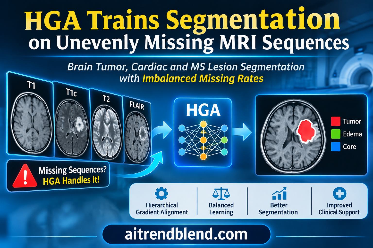
A patient with advanced kidney disease comes in for a brain tumor follow up. The care team decides against gadolinium contrast, so the scan has no contrast enhanced T1 image, the sequence that best shows an actively growing tumor. In the next room, a patient who cannot stay still through the full protocol finishes without a FLAIR scan. Neither situation is unusual, and both leave a segmentation model with fewer inputs than it was designed for.
A team at Huazhong University of Science and Technology in Wuhan argues that the usual fix for this problem is trained on the wrong kind of missing data. Their method, Hierarchical Gradient Alignment, or HGA, treats every combination of available sequences as its own task and balances them during training. The results are strong. The more useful story is where HGA wins, where it quietly gives ground, and which of its parts carry the gains.
Key points
- Most methods for missing MRI sequences are trained by hiding inputs at random with equal odds. HGA is built for imperfect data, where some sequences are missing far more often than others and stay missing for that patient.
- It combines three ideas. Training runs on shuffled sequences that sample every combination of inputs equally, each single sequence branch learns from the fused prediction, and per sequence weights shift according to how well each branch is learning.
- Across six imbalanced settings on BraTS2020 brain tumors, HGA averaged 70.24 Dice against 68.81 for PASSION, the strongest baseline. On MyoPS2020 heart scans the figures were 73.82 and 71.96. Both averages are our arithmetic from the paper’s Table IV.
- HGA had the best Dice in all 12 settings but the best Hausdorff distance in only 6, so boundary accuracy is roughly a tie with PASSION.
- Its gains are uneven by design. They are largest for inputs that include the rare FLAIR and T2 sequences, and it trails on combinations of the common sequences alone.
- All missingness was simulated by masking complete scans, the cardiac test set has 22 slices, and the paper reports no reader study. This is solid methods research, not clinical evidence.
Medical disclaimer. This article explains published research on medical image segmentation. It is not medical advice, diagnosis or treatment, and it does not evaluate any approved clinical product. Software that outlines tumors or lesions on patient scans must be validated and supervised by qualified professionals. If you have questions about your own imaging, please talk to your care team.
Why missing sequences are hard for segmentation models
An MRI exam for a brain tumor is usually several scans, not one. Each sequence makes different tissue stand out. T1 weighted images give anatomy, contrast enhanced T1, written T1c, lights up the part of the tumor that is actively growing, FLAIR shows the swelling around it, and T2 separates fluid from tissue. The BraTS benchmarks, described by Menze and colleagues in IEEE Transactions on Medical Imaging, ask a model to outline three nested regions from all four. Those are the whole tumor, the tumor core and the enhancing tumor.
Real exams often leave a sequence out. Protocols differ between hospitals, scanners have limits, patients move, and contrast is sometimes withheld for safety. The paper’s discussion cites consensus guidance on gadolinium use in patients with kidney disease and on more careful use of gadolinium in multiple sclerosis follow up. A model that only works when all four inputs are present is of limited use in that world.
The research field that tackles this is called incomplete multimodal learning. Methods fall into three families. Synthesis methods try to generate the missing scan. Distillation methods train a student for each subset of inputs using a teacher that sees everything. Shared representation methods map every sequence into one common feature space, so the model can work from whatever subset arrives. HeMIS from Havaei and colleagues was an early example of the shared approach, and mmFormer from Zhang and colleagues, which serves as HGA’s default backbone, is a widely used one. Our article on KEDR and diagnosis with a missing scan covers a related idea for classification.
Perfect data training versus imperfect data training
Here is the paper’s central complaint. Most of these methods are trained in what the authors call perfect data training. Every training case has all sequences, and the trainer hides some of them at random, with the same probability for each sequence, and a fresh draw at every iteration. A sequence hidden for a patient in one epoch reappears in the next.
Clinical data does not behave like that. A sequence that was never acquired never appears, and some sequences are missing far more often than others. The authors call this imperfect data training. Under it, a rare sequence is seen by the model on only a small fraction of patients, the same fraction every epoch, and the combinations that include it are rarer still.
“neither assumption reflects real clinical workflows”
Shi and colleagues, on equal and iteration varying masking in perfect data training
Two kinds of imbalance at once
The authors argue that imperfect data creates two imbalances. The first is between single sequences. A sequence that appears often dominates training, and the network’s features drift toward it while rarer sequences are neglected. This is the problem that methods such as OGM GE from Peng and colleagues address in general multimodal learning, and that PASSION, the same group’s ACM Multimedia 2024 method, addresses for medical segmentation.
The second imbalance is between combinations. With four sequences there are 15 non empty combinations. Under skewed missing rates, some of them, such as all four together, are common, and others, such as T2 alone, almost never appear in training. The paper’s point is that a combination can stay poorly trained even when each of its member sequences has been learned well, because the model never practiced fusing that particular set. Earlier work, PASSION included, did not address this second imbalance.
Availability and missing rates
$$ C \in \{0,1\}^{N \times M}, \qquad C_{nm} = 1 \text{ if sequence } m \text{ is available for case } n $$ $$ \mathcal{M}^m = \Big(N – \sum_{n} C_{nm}\Big) \big/ N $$Each row of \(C\) is one modality combination. With \(M\) sequences there are \(K = 2^M – 1\) combinations, and HGA treats each one as a task \(\mathcal{T}_k\).
How HGA works
HGA comes from Junjie Shi, Zhaobin Sun, Li Yu, Xin Yang and Zengqiang Yan at the School of Electronic Information and Communications, Huazhong University of Science and Technology. It is published in IEEE Transactions on Medical Imaging, volume 45, issue 6, and the authors state that their code is public. The method is a training scheme rather than a network, which is why it can be wrapped around different backbones. It has three parts, which the paper names out hierarchical alignment, in hierarchical alignment and dual hierarchical balancing.
Out hierarchical alignment, balancing the combinations
The first part deals with imbalance between combinations. Training cases are grouped by which sequences they have, giving one group per combination that actually occurs. Instead of sampling cases in proportion to how common they are, HGA samples every non empty group equally, draws cases inside a group uniformly with replacement, and shuffles the resulting mini batches into a sequence. A copy of the network trains on that sequence, one combination after another.
Why train in sequence rather than mix everything into one batch? The authors draw on meta learning. When a model takes a step on task one and then a step on task two, the second gradient is computed at a point the first task already moved, and the combined update implicitly rewards gradients of the two tasks that point the same way. The paper cites Dandi, Barba and Jaggi on implicit gradient alignment for this property, and the approximation it uses comes from Reptile, the first order meta learning method of Nichol, Achiam and Schulman.
The sequential objective
$$ \min_{\theta} \; \mathbb{E}_{\mathcal{T}_i \sim \mathcal{P}_M}\, \mathcal{L}(\mathcal{T}_i; \tilde{\theta}), \qquad \text{s.t.} \quad \tilde{\theta} = \min_{\theta} \; \mathbb{E}_{\mathcal{T}_j \sim \mathcal{I}(\mathcal{T}_i)}\, \mathcal{L}(\mathcal{T}_j; \theta) $$\(\mathcal{I}(\mathcal{T}_i)\) is the set of tasks that come before \(\mathcal{T}_i\) in the sampled sequence. Differentiating through this exactly would need second order gradients.
Second order gradients are expensive, so HGA uses the first order shortcut. After a copy of the network has trained through a sequence, the original weights move a fraction of the way toward the copy.
First order update after each sequence
$$ \tilde{\theta}_r \leftarrow \tilde{\theta}_r – \eta\, \nabla_{\tilde{\theta}_r} \mathcal{L}_n(x_n, y_n; \tilde{\theta}_r) \quad \text{for each mini batch in the sequence} $$ $$ \theta_r \leftarrow \theta_r + \epsilon_r\, \big(\tilde{\theta}_r – \theta_r\big) $$The paper raises \(\epsilon\) linearly from 0.1 to 1.0 over training. Cost grows with the number of sampled groups per sequence, not with the number of possible combinations.
In hierarchical alignment, teaching each sequence branch
The second part deals with imbalance between single sequences inside a combination. Backbones like mmFormer keep a separate encoder per sequence and fuse their features. HGA asks each single sequence branch to match the fused prediction, a form of self distillation. If knowledge distillation is new to you, our explainer on the mathematics of knowledge distillation is a good primer for the temperature scaled loss used here.
The detail that matters is what the teacher sees. The fused teacher receives exactly the sequences that the case has, and nothing more. Missing sequences stay masked for the teacher too, so it cannot pass along information from a scan that does not exist. The gap between a single branch and the fused branch then measures how much that sequence lags inside this particular combination.
Pixel wise self distillation
$$ \mathcal{L}^m_{pixel} = \frac{1}{I} \sum_{l=1}^{L} \sum_{i=1}^{I} \mathrm{KL}\!\left[ \sigma\!\Big(\frac{z^{m,l}_{n,i}}{\tau}\Big) \,\Big\|\, \sigma\!\Big(\frac{z^{t,l}_{n,i}}{\tau}\Big) \right] $$\(z^{m,l}_{n,i}\) is the output of the single sequence branch \(m\) at layer \(l\) for pixel \(i\), and \(z^{t,l}_{n,i}\) is the fused teacher’s. The temperature \(\tau\) is 4.
Pixel matching alone does not make the features of a weak sequence carry class meaning, so HGA adds a prototype loss. For each case and each sequence it averages the features of every class into a prototype, then asks each pixel’s feature to sit closest to its own class prototype, in relative terms through a cross entropy over distances, and in absolute terms through the distance itself. Prototypes as class anchors have a long history in medical segmentation, and our article on prototype guided graph reasoning for medical segmentation shows another use of them.
Class prototypes and the prototype loss
$$ c^m_n[k] = \frac{\sum_i z^{m,0}_{n,i}\, \mathbb{1}[y_{n,i} = k]}{\sum_i \mathbb{1}[y_{n,i} = k]}, \qquad D^m_{n,i}[k] = \big\lVert z^{m,0}_{n,i} – c^m_n[k] \big\rVert $$ $$ \mathcal{L}^m_{proto} = \sum_i \underbrace{-\log \frac{\exp(-D^m_{n,i}[y_{n,i}])}{\sum_k \exp(-D^m_{n,i}[k])}}_{\text{PRD}} + \lambda \underbrace{\big\lVert D^m_{n,i}[y_{n,i}] \big\rVert}_{\text{PAD}} $$PRD is the prototype relative distance and PAD the prototype absolute distance. The paper settles on \(\lambda = 0.001\).
Dual hierarchical balancing, deciding who needs help
The third part links the first two. For each case and each available sequence, HGA computes how well that sequence’s features cluster around the correct prototype, then compares it with the other available sequences of the same case. The result is a relative preference. A positive value means the sequence is ahead of its companions, a negative value means it lags.
Correct clustering score and relative preference
$$ S^m_n = \frac{\exp(-D^m_{n,i}[y_{n,i}])}{\sum_k \exp(-D^m_{n,i}[k])}, \qquad RP^m_n = C_{nm} \left\{ \frac{S^m_n \sum_{m} C_{nm}}{\sum_{m} \big(S^m_n C_{nm}\big)} – 1 \right\} $$Sample level preferences are noisy, so HGA averages them over all cases in the sequences of a training round to get a global preference per sequence. It then nudges a weight for each sequence, lowering it when the sequence is ahead and raising it when it lags, and projects the weights so they stay positive and keep a fixed overall size. Those weights scale the pixel distillation loss. A second switch, a mask that turns on only for a sequence with negative preference in that case, decides whether the prototype loss applies.
Global preference, weight update and mask
$$ \bar{RP}^m = \mathbb{E}_{\mathcal{T}_t \sim \mathcal{P}_M,\, n \sim \mathcal{T}_t} \big[ RP^m_n \big], \qquad \beta^m_r = \beta^m_{r-1} – \alpha\, \bar{RP}^m $$ $$ \boldsymbol{\beta}_r = \mathrm{Proj}_{\Gamma_\beta}(\boldsymbol{\beta}_r), \quad \Gamma_\beta = \big\{ \boldsymbol{\beta} \,:\, \beta^m \geq 0.1,\ \lVert \boldsymbol{\beta} \rVert_2 = \lVert \boldsymbol{\beta}_0 \rVert_2 \big\}, \qquad \delta^m_n = \mathbb{1}\big[RP^m_n < 0\big] $$Everything comes together in one loss per case. The backbone’s own segmentation loss on the fused prediction is joined by the distillation and prototype terms for every available sequence.
The full objective for case n
$$ \mathcal{L}_n = \mathcal{L}_{seg}(C_n x_n, y_n) + \sum_{m=1}^{M} C_{nm} \big( \lambda_1 \beta^m \mathcal{L}^m_{pixel} + \lambda_2\, \delta^m_n\, \mathcal{L}^m_{proto} \big) $$The paper uses \(\lambda_1 = 0.5\) and \(\lambda_2 = 0.02\).
Key takeaway
HGA is a training recipe, not an architecture. Combinations get equal turns, each sequence branch is coached by the fused prediction it belongs to, and per sequence weights move toward whichever branch is falling behind. Because no layer changes, the recipe can wrap other backbones.
How the experiments were set up
Three public MRI benchmarks are used. BraTS2018 and BraTS2020 supply brain tumor scans with T1, T1c, FLAIR and T2. BraTS2020’s 369 cases split into 219 for training, 50 for validation and 100 for testing, by official case identifiers. MyoPS2020 supplies cardiac MRI from 25 patients with three sequences, bSSFP for anatomy, LGE for scar and T2 for swelling, and asks for the left and right ventricular blood pools and the myocardium. The paper lists it as 102 slices split 80 for training and 22 for testing. MSSEG2016 supplies multiple sclerosis lesion data from six centers with up to five sequences, listed as 2685 slices split 1822, 123 and 740. For external validation, the BraTS2020 model is tested on BraTS2023 after removing cases that overlap with BraTS2020, leaving 886.
Imperfect data is simulated by masking whole sequences per case according to fixed, unequal missing rates, so a sequence masked for a case stays masked. For the main comparison, the brain tumor missing rates take values of 0.2, 0.5 and 0.8 in six orders, with T1 and T1c sharing a rate, and the cardiac rates take 0.3, 0.5 and 0.7 in six orders. Other experiments use rates of 0.1, 0.3, 0.7 and 0.9 for T1, T1c, FLAIR and T2, where FLAIR and T2 are rare.
The default backbone is mmFormer, trained with AdamW at a learning rate of 0.0002, weight decay 0.0001 and a batch size of one, for 300 epochs on NVIDIA RTX 3090 GPUs. Brain volumes are trained in 3D with 80 cubed crops and cardiac and lesion data in 2D. HGA runs 300 rounds of 15 sequences each. Baselines include medical balancing methods GSS, MAG, GMD, MetaMAR and PASSION, general balancing methods ModDrop, PMR, BML, AGM and Re-Learning, and multitask learning methods HPS, DWA, PCGrad, GradNorm, MGDA and uncertainty weighting. Results are reported as Dice in percent and Hausdorff distance in millimetres, computed per subject and averaged over all modality combinations.
What the numbers show
| Setting | BraTS Baseline | BraTS PASSION | BraTS HGA | MyoPS Baseline | MyoPS PASSION | MyoPS HGA |
|---|---|---|---|---|---|---|
| Perfect data, no missing | 70.58 / 14.68 | 74.27 / 9.66 | ||||
| (s, m, l) | 67.66 / 14.35 | 69.31 / 10.52 | 70.34 / 12.15 | 68.81 / 21.11 | 73.28 / 14.50 | 73.63 / 14.58 |
| (s, l, m) | 66.43 / 17.10 | 69.37 / 9.64 | 70.20 / 10.50 | 65.29 / 27.99 | 71.99 / 15.79 | 73.34 / 14.77 |
| (m, s, l) | 67.95 / 19.44 | 68.90 / 10.37 | 70.92 / 10.51 | 67.89 / 20.49 | 73.21 / 14.79 | 74.82 / 15.11 |
| (m, l, s) | 67.23 / 16.86 | 69.06 / 12.21 | 69.97 / 11.52 | 64.61 / 23.98 | 69.91 / 17.65 | 71.48 / 15.22 |
| (l, s, m) | 66.59 / 15.49 | 68.31 / 11.44 | 70.29 / 10.48 | 67.19 / 21.97 | 71.49 / 16.86 | 74.84 / 16.06 |
| (l, m, s) | 66.80 / 16.62 | 67.91 / 11.71 | 69.70 / 11.17 | 69.09 / 16.70 | 71.86 / 14.97 | 74.80 / 15.02 |
| Mean of six, our arithmetic | 67.11 / 16.64 | 68.81 / 10.98 | 70.24 / 11.05 | 67.15 / 22.04 | 71.96 / 15.76 | 73.82 / 15.13 |
On Dice, HGA wins every one of the 12 settings. Averaged over the six orders, it leads the mmFormer baseline by 3.13 points on BraTS2020 and 6.67 points on MyoPS2020, and it leads PASSION by 1.43 and 1.86 points, all by our arithmetic from Table IV. The per setting lead over PASSION ranges from 0.83 to 2.02 points on brain tumors and from 0.35 to 3.35 points on hearts. Simpler balancing schemes fare worse. The authors note that ModDrop, PMR, GMD and MetaMAR degrade noticeably when one sequence dominates training.
Hausdorff distance tells a more mixed story. HGA has the best average boundary error in 6 of the 12 settings, and PASSION has it in the other 6. On BraTS2020 the six setting means are 11.05 mm for HGA and 10.98 mm for PASSION, a tie. A pattern sits in the brain tumor rows that the paper does not discuss. PASSION keeps the better boundary in both settings where T1 and T1c are the most available inputs, and HGA has the better boundary in both settings where they are the rarest. The authors explain the general tradeoff themselves. PASSION estimates preferences case by case, which can sharpen edges, while HGA smooths its estimates over whole sequences of cases and sometimes fits boundaries less aggressively.
One more detail stands out. On MyoPS2020, HGA trained with missing sequences scores higher than the baseline trained on complete data in three settings, reaching 74.84 against 74.27. That does not mean missing data helps. It means the baseline trained on complete data is not the ceiling, because it lacks HGA’s extra training signals. The cardiac test set also holds only 22 slices, so differences of half a point are fragile.
Where the gains come from
Table XI of the paper breaks the BraTS2020 result down by combination, with rates of 0.1, 0.3, 0.7 and 0.9 for T1, T1c, FLAIR and T2. HGA has the best average on all three tumor regions, at 83.71 for whole tumor, 71.49 for tumor core and 54.36 for enhancing tumor, against 82.11, 70.15 and 52.68 for PASSION. The paper reports paired Wilcoxon signed rank tests that put every comparison of averages below p of 0.001.
The average hides a pattern, shown in the feature chart above. We averaged the three regions per combination for HGA and for PASSION. HGA’s largest gains come from combinations that include a rare sequence, 3.95 points for FLAIR with T2, 3.10 for FLAIR alone and 2.54 for T2 alone. It loses on exactly two combinations, T1c alone by 1.14 points and T1 with T1c by 1.42 points. These are the two inputs that rely on T1c without FLAIR or T2. Across the 45 cells of the table, HGA is not the best in 12, and every one of those 12 cells includes T1c.
That is the expected price of a method that gives rare combinations equal turns. The common combinations get fewer turns than their share of the data, and the strongest single sequence for the enhancing tumor gets less specialized attention. Whether that trade is good depends on the clinic. Where T1c is almost always acquired, the combinations HGA is weakest on are the ones that will arrive most often.
Key takeaway
HGA moves performance toward rare combinations. It gains up to 3.95 Dice points where FLAIR or T2 is present and loses up to 1.42 points where T1c carries the case alone. The average improves, but the distribution of quality across patients changes too.
When one sequence almost never appears
The most dramatic test removes FLAIR from training at rising rates while every other sequence is always available, then evaluates the model on FLAIR alone. At a 99 percent missing rate, FLAIR appears in roughly 2 of the 219 training volumes, by our arithmetic.
| FLAIR missing rate | Baseline | MetaMAR | HGA |
|---|---|---|---|
| 0 | 59.61 / 20.62 | 60.73 / 17.75 | 62.88 / 12.08 |
| 0.5 | 57.07 / 24.31 | 58.53 / 16.32 | 60.37 / 11.46 |
| 0.95 | 38.05 / 52.84 | 47.43 / 30.36 | 52.27 / 19.19 |
| 0.99 | 32.30 / 67.67 | 37.92 / 42.07 | 46.54 / 28.07 |
At 99 percent missing, HGA’s FLAIR only Dice of 46.54 is 14.24 points above the baseline and 8.62 above MetaMAR, which uses meta gradients to reduce bias toward frequent sequences. Its Hausdorff distance is less than half the baseline’s. It is still 16.34 points below its own result when FLAIR is always present, so a nearly absent sequence remains a real handicap. Still, a model that degrades this gracefully from two examples is a meaningful result.
External data, calibration and other backbones
Trained on BraTS2020 and tested on the 886 deduplicated BraTS2023 cases, mmFormer with HGA reaches 73.40 Dice, against 71.51 with PASSION and 69.83 for plain mmFormer. Boundary error and expected calibration error also improve, 11.06 mm and 0.0836 against 11.66 mm and 0.0871 for PASSION. Two general segmentation networks not designed for missing inputs, SwinUNETR and nnUNet, trail at 66.14 and 68.76. All methods score higher on BraTS2023 than on their own BraTS2020 test set, which suggests the external set is easier rather than harder, so this is a useful check of stability more than a stress test of generalization.
Calibration is reported for 15 combinations against multitask and balancing methods. HGA has the lowest average expected calibration error for all three regions, and the largest margins appear in the T2 only and FLAIR only settings, where competitors tend to be overconfident. A risk coverage analysis in the paper points the same way. When the least confident predictions are set aside, HGA makes the fewest errors on the rest.
The paper also wraps HGA around RFNet, M2FTrans, Shaspec and a Dynamic Sharing framework on BraTS2018 and BraTS2020, and around SwinUNETR, nnUNet and mmFormer at two batch sizes. The plotted results show gains for every backbone, including about 3.45 Dice points on SwinUNETR and 3.63 on nnUNet at a batch size of one. Exact numbers for the other backbones are given only as bar charts.
Against general multitask learning
If each combination is a task, why not use a standard multitask optimizer? The authors compare HGA with six multitask optimizers and three general balancing methods on the same Dynamic Sharing backbone. The optimizers include PCGrad from Yu and colleagues, GradNorm from Chen and colleagues and MGDA from Sener and Koltun.
| Method | T1 only | T1c only | FLAIR only | T2 only | All four | Average of 15 |
|---|---|---|---|---|---|---|
| HPS | 53.98 | 75.18 | 57.64 | 57.15 | 70.71 | 65.76 |
| PCGrad | 53.89 | 75.97 | 57.28 | 55.90 | 70.76 | 65.67 |
| GradNorm | 53.42 | 74.44 | 56.94 | 56.89 | 70.53 | 65.36 |
| Uncertainty weighting | 53.22 | 76.29 | 57.42 | 56.57 | 71.50 | 66.13 |
| BML | 54.46 | 75.76 | 57.92 | 56.72 | 71.98 | 66.51 |
| HGA | 53.02 | 74.46 | 58.77 | 58.12 | 76.55 | 68.54 |
| GradNorm with HGA | 51.09 | 74.29 | 57.52 | 57.82 | 79.06 | 68.70 |
HGA’s average of 68.54 is 2.03 points above the strongest competitor, BML, a general balancing method. Its biggest gain is on all four sequences together, 76.55 against 71.98. On T1 alone and T1c alone, the two most available sequences in this setting, it scores below most competitors, 1.44 points behind BML on T1 and 1.83 behind uncertainty weighting on T1c. The same trade appears when HGA is added to a multitask optimizer. GradNorm with HGA reaches the best average of all at 68.70, but adding HGA to PCGrad costs 5.42 points on T1 alone and 3.55 on T1c alone. The authors acknowledge the pattern, writing that HGA may down weight abundant sequences while gaining more on scarce ones.
On MSSEG2016, with five sequences, 31 combinations and missing rates from 0.9 for gadolinium enhanced T1 down to 0.1 for FLAIR, HGA averages 52.10 Dice against 45.20 for BML, a 6.90 point lead. It is the best method on every combination the paper shows. That comparison includes multitask and general balancing methods, though, not PASSION or other methods built for missing sequences, so it shows that HGA beats general optimizers rather than its closest competitors on this dataset.
What the ablations reveal
All ablations run on BraTS2020 with missing rates of 0.2, 0.4, 0.6 and 0.8 for T1, T1c, FLAIR and T2, where the mmFormer baseline averages 66.19 Dice and 20.82 mm.
| Variant | Dice | HD | Dice change |
|---|---|---|---|
| Baseline, mmFormer | 66.19 | 20.82 | |
| Pixel self distillation only | 68.60 | 11.54 | +2.41 |
| Prototype loss only | 67.16 | 19.97 | +0.97 |
| Out hierarchical alignment only | 68.23 | 21.28 | +2.04 |
| Both distillation terms | 69.09 | 11.91 | +2.90 |
| Both distillation terms and alignment | 69.56 | 11.30 | +3.37 |
| Full HGA, adding balancing | 70.50 | 11.41 | +4.31 |
| Plain resampling instead | 66.40 | 23.56 | +0.21 |
| MAML instead | 67.93 | 16.00 | +1.74 |
| PASSION | 69.78 | 11.68 | +3.59 |
Three things stand out. First, the single biggest contributor is pixel wise self distillation, worth 2.41 Dice points on its own and responsible for nearly all of the boundary improvement, cutting Hausdorff distance from 20.82 to 11.54 mm. Second, out hierarchical alignment on its own adds 2.04 Dice points but slightly worsens the boundary, from 20.82 to 21.28 mm. Its boundary benefit appears only together with distillation. Third, the balancing step adds 0.94 Dice points on top of everything else and leaves the boundary slightly worse, 11.41 against 11.30 mm. Plain resampling, the obvious alternative to balanced sequences, adds only 0.21 points and makes boundaries worse, which supports the authors’ view that reweighting alone does not resolve the conflict. Swapping in MAML, the meta learning method of Finn, Abbeel and Levine, gives 67.93, below the first order Reptile style update that HGA uses.
The out hierarchical row in Table V is identical to the Reptile row in Table VI, which confirms that this component is a Reptile style update applied to combination grouped sequences. There is a subtlety the paper does not discuss. Because \(\epsilon\) rises to 1.0 by the end of training, the final rounds simply replace the original weights with the trained copy, which is ordinary sequential training on group balanced sequences. With a batch size of one, the line between that and balanced resampling is thinner than the framing suggests. The ablation shows a real gap between the two, 68.23 against 66.40 Dice, but it does not isolate how much of it comes from the early rounds where \(\epsilon\) is small.
The balancing weights do not favor rare sequences
Table IX of the paper lists the learned sequence weights after training with missing rates of 0.1, 0.3, 0.7 and 0.9 for T1, T1c, FLAIR and T2. With the default settings, the weights end at 1.34 for T1, 1.16 for T1c, 0.57 for FLAIR and 0.74 for T2. The common sequences get the higher weights and the rare ones the lower.
A reader who expects the balancing step to push the rare sequences will find it does roughly the opposite. Our reading is that the preference score tracks how well a sequence’s features separate the classes, not how often it appears. FLAIR and T2 show edema and the whole tumor clearly, so their features cluster well and register as ahead. T1 carries little tumor contrast, so it registers as lagging and gets more distillation. The help for rare sequences comes from the group balanced sequences instead. This is consistent with the paper’s design, but the paper does not spell it out, and it is worth knowing before tuning the method. Our toy run in the code section shows the same direction.
Settings that matter less, and one that matters more
The method is not fragile. Across norms, floors, smoothing rates and masking schemes in Table IX, average Dice stays between 69.50 and 70.22, and every setting stays above PASSION’s 68.01 under the same missing rates. The paper’s own sensitivity study finds the best region near \(\lambda_1 = 0.5\) and \(\lambda_2\) between 0.02 and 0.1, with a temperature near 4. Interestingly, the default configuration is not the best one in these sweeps. An L2 floor of 0.7 gives 70.22 against 69.85 for the default floor of 0.1.
The sequence construction matters more. Table XII compares ways of ordering the training sequences. A variant the authors call Group Mini Sequence, which draws a short run from one group and appends the full combination, reaches 70.25 Dice and 10.99 mm, against 69.69 and 11.83 for the default random order. The authors suggest it works because it revisits the complete combination more often. It is an obvious upgrade for anyone reimplementing the method.
Cost
On the Dynamic Sharing backbone, HGA trains in 5.56 hours with 7536 MiB of GPU memory. That is cheaper than PASSION at 6.73 hours and 9116 MiB, and well below Re-Learning at 7.17 hours and 12650 MiB. Removing out hierarchical alignment saves only 20 MiB and 0.07 hours, so the balanced sequences are nearly free. The fastest multitask baseline, HPS, needs 3.50 hours and 6576 MiB. Inference is unchanged, because HGA only alters training.
Clinical translation gap
How far is this from a clinic? Further than the tables suggest, for reasons worth spelling out.
The missing data is simulated. Every benchmark here starts from complete scans, and sequences are removed at random according to fixed rates. That makes missingness independent of the patient. In real practice it is not. Contrast is withheld from patients with poor kidney function, sequences are cut short in patients who cannot lie still, and protocols vary with the clinical question. The paper’s own clinical motivation describes exactly these patterns. A model trained under random masking may face a different mix of patients for each combination in deployment, for example more frail patients among scans without T1c, and its accuracy on those groups is untested.
The evaluation is overlap and boundary metrics only. There is no reader study, no measurement of tumor volumes, and no link to treatment decisions. Small Dice differences on the enhancing tumor, the region with the lowest scores across all methods, may or may not change a clinical assessment.
The losses on T1c centered combinations matter in practice. In many brain tumor protocols, contrast enhanced T1 is the sequence most consistently acquired, so a clinic would see those combinations often. HGA’s average gain partly comes at their expense.
The cardiac and lesion results rest on thin data. The MyoPS2020 test set is 22 slices with no validation set, and the paper does not say whether its 2D splits for MyoPS2020 and MSSEG2016 were made by patient or by slice. If slices from one patient appear in both training and testing, scores would be inflated for every method.
Regulatory and safety note, our reading
Software that segments tumors or lesions for clinical use is regulated as a medical device in most jurisdictions. A method that performs differently depending on which sequences were acquired raises a specific safety question, whether performance on each combination is acceptable on its own, not just on average. Any clinical path would need validation on scans with naturally missing sequences, reporting by combination and by patient group, review of outputs by qualified staff, and the usual approval route for the device that wraps the model.
Limitations, sample size and bias
- Simulated missingness. All missing sequences are produced by masking complete scans at random, which assumes missingness unrelated to the patient. Real missingness is often driven by the patient’s condition.
- Small test sets for two tasks. MyoPS2020 is tested on 22 slices from 25 patients in total, and the paper does not state whether the 2D splits for MyoPS2020 and MSSEG2016 are by patient.
- Pooled significance tests. The Wilcoxon tests in Table XI cover 100 test cases across 15 combinations. Results from the same patient across combinations are correlated, so the very small p values likely overstate how independent the evidence is. This is our inference, not a point the paper makes.
- Unstated spread. Table XI reports variation across cases, but the later tables on sequence order, external data, multitask methods and MSSEG2016 report plus or minus values without saying whether they come from repeated runs, seeds or cases, and no random seeds are stated. The same default configuration appears as 69.85 Dice in Tables IX and XI and as 69.69 in Tables XII and XIV, which suggests single runs in some tables and averages in others.
- Selection on the evaluated data. The ablations and hyperparameter sweeps are reported on BraTS2020, and the paper does not say whether the validation or test split was used for them.
- Uneven gains. HGA trails on combinations of the common sequences, including T1c alone and T1 with T1c, and its boundary accuracy is no better than PASSION’s on average.
- Narrow baselines on MSSEG2016. The multiple sclerosis comparison includes multitask and general balancing methods, not PASSION or other methods built for missing sequences.
- Dataset bias. BraTS, MyoPS and MSSEG are curated research collections. Performance on other vendors, field strengths, pediatric patients or other diseases is unknown.
- Scope. The authors note that HGA is evaluated only for segmentation and does not model how hard individual cases are, and they list both as future work.
What practitioners can take from this
If you train on clinical data with missing sequences, start by measuring it. Count how often each combination occurs and evaluate per combination, not only on average. HGA’s per combination results show how much an average can hide.
If you want one component, take the pixel self distillation with a teacher restricted to the same inputs. In the ablation it gives most of the Dice gain and nearly all of the boundary gain, and it needs no change to sampling. Then try group balanced sequences, using the Group Mini Sequence order from Table XII. Treat the balancing weights as a measure of feature quality, not of rarity, and inspect them after training.
If you compare methods for missing inputs, report Hausdorff distance next to Dice, list results for every combination, and state how test splits relate to patients. Related work on this site handles missing inputs differently. Our article on contrast free tumor AI and its text model looks at models built for scans acquired without contrast, and our piece on ETF-UML and incomplete ICU data takes a fusion approach for clinical records. More studies of this kind sit in our Medical AI section.
Conclusion
HGA is a careful answer to a problem that most missing sequence research had set aside. Training data in hospitals is not missing at random with equal odds. Some sequences are rare, and the combinations they form are rarer still. By giving every combination equal turns, distilling each sequence branch from the fused prediction it belongs to, and reweighting branches by how well they learn, HGA beats every baseline the authors tested on Dice, in all 12 main settings across brain tumors and hearts, and on external BraTS2023 data, at lower training cost than its closest competitor.
The conceptual shift is to treat each combination of inputs as its own task. That reframing explains why a model can know every sequence well and still fuse a rare combination badly, and it opens the problem to tools from meta learning and multitask optimization. The paper shows HGA can sit alongside those tools rather than replace them.
The per combination results sharpen what that shift costs. Gains concentrate where the rare FLAIR and T2 sequences are present, and the method gives ground where T1c works without them. The learned weights favor sequences whose features lag, not sequences that are rare. Boundary accuracy is roughly tied with PASSION. None of this undermines the method, but it should shape how it is deployed and evaluated.
The remaining limits are familiar for this field. Missingness is simulated from complete scans, so it ignores why sequences go missing in real patients. The cardiac test set is tiny, the 2D splits are not clearly by patient, the significance tests pool correlated results, and there is no reader study. The authors themselves point to classification and detection tasks and to difficulty aware weighting as next steps.
The most convincing next experiment would use a dataset where sequences are missing for real clinical reasons, report results for every combination and patient group, and include radiologist review of the cases where HGA and its competitors disagree. That would show whether rebalancing toward rare combinations helps the patients who actually arrive with them.
A model is only as fair as the data it practices on, and HGA’s lesson is that fairness across inputs has to be built into training rather than hoped for at test time.
A reference implementation in PyTorch
The paper points to the authors’ GitHub repository, and that is the version to use for any real comparison. The listing below is our own editorial reconstruction, written to make every equation runnable. It draws a fixed availability matrix from imbalanced missing rates, builds a small 2D multimodal segmenter in the spirit of mmFormer, and implements pixel self distillation, class prototypes with the PRD and PAD loss, the correct clustering score, relative and global preferences, the projected weight update and mask, the full loss, the group balanced sequences with the first order update, a baseline with the same number of gradient steps, and Dice on all 15 combinations.
We ran the listing on a CPU with 400 synthetic training images of four channels and target missing rates of 0.1, 0.3, 0.7 and 0.9, which came out at 0.07, 0.24, 0.67 and 0.88 in the drawn sample. Fourteen of the 15 combinations occurred, the smallest with a single image. Both models took 672 gradient steps. The result is honest rather than flattering. The baseline averaged 0.903 Dice over the 15 combinations and our HGA reconstruction 0.862, lower on 14 combinations and tied on one. The learned weights did move in the direction of the paper’s Table IX, rising for the two common channels and falling for the rarest, to 1.007, 1.013, 1.003 and 0.977.
We read the gap as a property of the toy rather than of the method. It runs 12 rounds instead of 300, the small early values of \(\epsilon\) discard much of what each sequence learns, and equal sampling of groups replays the single image group many times. Two extra runs support that reading. With \(\epsilon\) fixed at 1, the same run reaches 0.907, level with the baseline, while group balanced sequences with only the plain segmentation loss reach 0.889. A second seed moves our default run from 0.862 to 0.894 and the baseline from 0.903 to 0.900, so differences of a few hundredths in a toy this small say little about the method. Treat the listing as a way to read the equations, and use the authors’ repository for anything you would report.
"""
HGA reference sketch in PyTorch
===============================
An editorial reconstruction of Hierarchical Gradient Alignment (HGA) from
Shi, Sun, Yu, Yang and Yan, "Addressing Imbalanced Modal Incompleteness in
Realistic Multi-Modal Medical Image Segmentation via Hierarchical Gradient
Alignment", IEEE Transactions on Medical Imaging 45(6), 2026, pages 3066 to
3081, DOI 10.1109/TMI.2026.3667605. This is NOT the authors' code. The paper
points to github.com/Jun-Jie-Shi/HGA for the official implementation.

What is here
  * Imperfect data training: a fixed availability matrix C (N x M) drawn
    once from imbalanced missing rates, so a missing modality stays
    missing for that sample all through training
  * A small 2D multimodal segmenter in the spirit of mmFormer: one encoder
    per modality, masked fusion, a shared decoder with two output levels,
    and unimodal branches that reuse the decoder
  * Pixel wise self distillation from the fused teacher to each unimodal
    student at every output level                                      Eq. 2
  * Class prototypes per sample and modality, PRD + PAD prototype loss  Eq. 3-4
  * Correct clustering score, relative preference, global preference,
    projected update of the modality weights beta, mask delta          Eq. 5-8
  * Total sample loss                                                   Eq. 9
  * Out hierarchical alignment (Algorithm 1): group samples by modality
    combination, sample groups uniformly, shuffle into sequences, train a
    cloned model on each sequence, then move the slow weights by
    epsilon * (fast - slow), a first order (Reptile style) update
  * A plain baseline with the same number of gradient steps
  * Dice on all 2^M - 1 modality combinations, and a CPU smoke test

Simplifications, stated plainly
  * Tiny 2D network and synthetic four channel data instead of mmFormer on
    BraTS. The point is to make every equation runnable, not to match the
    paper's numbers.
  * Mini batches hold samples from one combination group. The paper uses a
    batch size of one.
  * The teacher logits are detached in the distillation loss and S_n^m is
    averaged over labelled pixels. The paper does not state either choice.
  * The projection onto {beta >= beta_min, ||beta||_2 = ||beta_0||_2} is an
    iterative clamp and rescale, which is our approximation.
"""
import itertools
import math
import random
import time
import torch
import torch.nn as nn
import torch.nn.functional as F


# ---------------------------------------------------------------------------
# 1. Imperfect data training setup
# ---------------------------------------------------------------------------
def draw_availability(n, missing_rates, gen):
    """C[n, m] = 1 if modality m is available for sample n. Drawn once and
    kept fixed, which is the imperfect data training (IDT) setting. Samples
    with no modality left are redrawn."""
    M = len(missing_rates)
    C = torch.zeros(n, M)
    p_keep = 1 - torch.tensor(missing_rates)
    for i in range(n):
        while True:
            row = (torch.rand(M, generator=gen) < p_keep).float()
            if row.sum() > 0:
                break
        C[i] = row
    return C


def empirical_missing_rate(C):
    """M^m = (N - sum_n C_nm) / N."""
    return 1 - C.mean(0)


def all_combinations(M):
    """The 2^M - 1 non empty modality subsets, each treated as a task."""
    combos = []
    for k in range(1, M + 1):
        for subset in itertools.combinations(range(M), k):
            v = torch.zeros(M)
            v[list(subset)] = 1
            combos.append(v)
    return combos


def group_by_combination(C):
    """Out hierarchical grouping {D_T_k}: indices of samples per combination."""
    groups = {}
    for i, row in enumerate(C):
        key = tuple(int(x) for x in row.tolist())
        groups.setdefault(key, []).append(i)
    return groups


# ---------------------------------------------------------------------------
# 2. A small multimodal segmenter
# ---------------------------------------------------------------------------
class ModalEncoder(nn.Module):
    def __init__(self, ch=24):
        super().__init__()
        self.net = nn.Sequential(
            nn.Conv2d(1, ch, 3, padding=1), nn.GroupNorm(4, ch), nn.GELU(),
            nn.Conv2d(ch, ch, 3, stride=2, padding=1), nn.GroupNorm(4, ch), nn.GELU(),
            nn.Conv2d(ch, ch, 3, padding=1), nn.GroupNorm(4, ch), nn.GELU())

    def forward(self, x):
        return self.net(x)


class SharedDecoder(nn.Module):
    """Returns logits at two levels (coarse, full) and the full resolution
    feature map that feeds the prototype loss (the paper's layer l = 0)."""

    def __init__(self, ch=24, n_cls=3):
        super().__init__()
        self.coarse = nn.Sequential(nn.Conv2d(ch, ch, 3, padding=1), nn.GELU())
        self.head_coarse = nn.Conv2d(ch, n_cls, 1)
        self.fine = nn.Sequential(nn.Conv2d(ch, ch, 3, padding=1), nn.GELU(),
                                  nn.Conv2d(ch, ch, 3, padding=1), nn.GELU())
        self.head_fine = nn.Conv2d(ch, n_cls, 1)

    def forward(self, f, out_size):
        h = self.coarse(f)
        logit_c = self.head_coarse(h)
        h = F.interpolate(h, size=out_size, mode="bilinear", align_corners=False)
        feat0 = self.fine(h)
        logit_f = self.head_fine(feat0)
        return [logit_f, logit_c], feat0


class MultiModalSegmenter(nn.Module):
    def __init__(self, M=4, ch=24, n_cls=3):
        super().__init__()
        self.M = M
        self.encoders = nn.ModuleList([ModalEncoder(ch) for _ in range(M)])
        self.fuse = nn.Conv2d(ch + M, ch, 1)
        self.decoder = SharedDecoder(ch, n_cls)

    def forward(self, x, C):
        """x (B,M,H,W) with missing channels zeroed, C (B,M) availability.
        Encoded features of missing modalities are set to zero, as in the
        paper's IDT emulation. Returns fused outputs and per modality outputs."""
        B, M, H, W = x.shape
        feats = [enc(x[:, m:m + 1]) * C[:, m].view(B, 1, 1, 1)
                 for m, enc in enumerate(self.encoders)]
        stack = torch.stack(feats, 1)                               # (B,M,ch,h,w)
        denom = C.sum(1).clamp_min(1).view(B, 1, 1, 1)
        fused = stack.sum(1) / denom                                # masked mean
        h, w = fused.shape[-2:]
        cond = C.view(B, M, 1, 1).expand(B, M, h, w)
        fused = F.gelu(self.fuse(torch.cat([fused, cond], 1))) + fused
        fused_logits, fused_feat = self.decoder(fused, (H, W))
        uni = [self.decoder(f, (H, W)) for f in feats]              # students
        return fused_logits, fused_feat, uni


# ---------------------------------------------------------------------------
# 3. Losses
# ---------------------------------------------------------------------------
def dice_ce_loss(logits, y, n_cls):
    ce = F.cross_entropy(logits, y)
    p = logits.softmax(1)
    oh = F.one_hot(y, n_cls).permute(0, 3, 1, 2).float()
    inter = (p * oh).sum((0, 2, 3))
    dice = 1 - (2 * inter + 1) / (p.sum((0, 2, 3)) + oh.sum((0, 2, 3)) + 1)
    return ce + dice[1:].mean()


def seg_loss(levels, y, n_cls):
    """Deep supervision over output levels, coarse levels use a nearest
    downsampled label map."""
    loss = 0.0
    for lg in levels:
        yy = y if lg.shape[-1] == y.shape[-1] else \
            F.interpolate(y[:, None].float(), size=lg.shape[-2:], mode="nearest")[:, 0].long()
        loss = loss + dice_ce_loss(lg, yy, n_cls)
    return loss / len(levels)


def pixel_self_distillation(student_levels, teacher_levels, tau=4.0):
    """Eq. 2. (1/I) sum_l sum_i KL[ sigma(z^m / tau) || sigma(z^t / tau) ],
    with the KL taken in the order the paper writes it. Returns one value per
    sample (B,). The teacher is the fused branch fed with exactly the same
    modality set, so it carries no privileged information."""
    total = 0.0
    for zs, zt in zip(student_levels, teacher_levels):
        ps = F.log_softmax(zs / tau, 1)
        pt = F.log_softmax(zt.detach() / tau, 1)
        kl = (ps.exp() * (ps - pt)).sum(1)                          # (B,h,w)
        total = total + kl.flatten(1).mean(1)
    return total


def class_prototypes(feat0, y, n_cls):
    """Eq. 3. c^m_n[k] = mean of layer 0 features over pixels of class k.
    Returns (B,K,ch) prototypes and a (B,K) mask of classes present."""
    oh = F.one_hot(y, n_cls).permute(0, 3, 1, 2).float()           # (B,K,H,W)
    cnt = oh.sum((2, 3))                                            # (B,K)
    proto = torch.einsum("bkhw,bchw->bkc", oh, feat0) / cnt.clamp_min(1)[..., None]
    return proto, cnt > 0


def prototype_terms(feat0, y, n_cls, lam=1e-3):
    """Eq. 4 and Eq. 5. D[k] = || z_i - c[k] ||. PRD is cross entropy over -D,
    PAD is lambda * D[y]. S is the softmax score of the true class, averaged
    over pixels, which is the correct clustering score of Eq. 5."""
    proto, present = class_prototypes(feat0, y, n_cls)
    B, ch, H, W = feat0.shape
    z = feat0.permute(0, 2, 3, 1).reshape(B, H * W, ch)
    D = torch.cdist(z, proto)                                       # (B,HW,K)
    D = D.masked_fill(~present[:, None, :], 1e4)                    # absent classes
    yy = y.reshape(B, H * W)
    logp = F.log_softmax(-D, -1)
    prd = -logp.gather(-1, yy[..., None]).squeeze(-1)               # (B,HW)
    pad = D.gather(-1, yy[..., None]).squeeze(-1)
    loss = (prd + lam * pad).mean(1)                                # per sample
    score = logp.gather(-1, yy[..., None]).squeeze(-1).exp().mean(1)
    return loss, score


def relative_preference(S, C):
    """Eq. 6. RP^m_n = C_nm * ( S^m_n * sum_m C_nm / sum_m (S^m_n C_nm) - 1 ).
    Positive means modality m is ahead of the other available modalities for
    this sample, negative means it lags, zero means balanced or missing."""
    avail = C.sum(1, keepdim=True).clamp_min(1)
    mean_S = (S * C).sum(1, keepdim=True) / avail
    return C * (S / mean_S.clamp_min(1e-8) - 1)


def project_beta(beta, beta_min, target_norm, iters=20):
    """Approximate projection onto {beta >= beta_min, ||beta||_2 = target}."""
    b = beta.clone()
    for _ in range(iters):
        b = b.clamp_min(beta_min)
        free = b > beta_min + 1e-9
        fixed_sq = (b[~free] ** 2).sum()
        need = max(target_norm ** 2 - fixed_sq.item(), 1e-12)
        if free.any():
            b[free] = b[free] * math.sqrt(need / (b[free] ** 2).sum().item())
        if (b >= beta_min - 1e-9).all() and abs(b.norm().item() - target_norm) < 1e-6:
            break
    return b


class DualHierarchicalBalancer:
    """Eq. 7 and Eq. 8. Accumulates sample RP in a memory bank during a round,
    averages it into a global preference, and updates beta by a projected step."""

    def __init__(self, M, alpha=0.01, beta_min=0.1):
        self.beta = torch.ones(M)
        self.target = self.beta.norm().item()
        self.alpha, self.beta_min = alpha, beta_min
        self.bank = []

    def record(self, rp, C):
        self.bank.append((rp.detach(), C.detach()))

    def step(self):
        if not self.bank:
            return self.beta
        rp = torch.cat([r for r, _ in self.bank])
        c = torch.cat([c for _, c in self.bank])
        global_rp = (rp * c).sum(0) / c.sum(0).clamp_min(1)        # mean over available
        self.beta = project_beta(self.beta - self.alpha * global_rp, self.beta_min, self.target)
        self.bank = []
        return self.beta


def unimodal_seg_loss(levels, y, cm, n_cls):
    """Backbone level unimodal segmentation loss, on samples that have m."""
    keep = cm > 0
    if keep.sum() == 0:
        return 0.0
    return seg_loss([lg[keep] for lg in levels], y[keep], n_cls)


def hga_sample_loss(model, x, C, y, n_cls, balancer, lam1=0.5, lam2=0.02, tau=4.0, lam=1e-3):
    """Eq. 9 for a mini batch. L_seg on the fused output plus, for every
    available modality, lambda1 * beta^m * L_pixel + lambda2 * delta^m * L_proto.
    The backbone's own unimodal segmentation loss is kept, as mmFormer does."""
    fused_logits, _, uni = model(x, C)
    loss = seg_loss(fused_logits, y, n_cls)
    l_pix, l_pro, scores = [], [], []
    for m, (levels, feat0) in enumerate(uni):
        loss = loss + unimodal_seg_loss(levels, y, C[:, m], n_cls) / model.M
        l_pix.append(pixel_self_distillation(levels, fused_logits, tau))
        lp, sc = prototype_terms(feat0, y, n_cls, lam)
        l_pro.append(lp)
        scores.append(sc.detach())
    L_pix, L_pro, S = torch.stack(l_pix, 1), torch.stack(l_pro, 1), torch.stack(scores, 1)
    rp = relative_preference(S, C)                                  # Eq. 6
    delta = (rp < 0).float()                                        # Eq. 8, lagging modalities
    reg = (C * (lam1 * balancer.beta[None] * L_pix + lam2 * delta * L_pro)).sum(1).mean()
    balancer.record(rp, C)
    return loss + reg


def baseline_sample_loss(model, x, C, y, n_cls):
    """Backbone loss only, fused segmentation plus unimodal segmentation."""
    fused_logits, _, uni = model(x, C)
    loss = seg_loss(fused_logits, y, n_cls)
    for m, (levels, _) in enumerate(uni):
        loss = loss + unimodal_seg_loss(levels, y, C[:, m], n_cls) / model.M
    return loss


# ---------------------------------------------------------------------------
# 4. Training loops with an equal gradient step budget
# ---------------------------------------------------------------------------
def masked_batch(X, Y, C, idx):
    x = X[idx] * C[idx][..., None, None]
    return x, C[idx], Y[idx]


def train_baseline(model, X, Y, C, n_cls, steps, bs=8, lr=2e-3, seed=0):
    rng = random.Random(seed)
    opt = torch.optim.AdamW(model.parameters(), lr=lr, weight_decay=1e-4)
    N = len(X)
    for _ in range(steps):
        idx = rng.sample(range(N), bs)                              # follows empirical frequencies
        x, c, y = masked_batch(X, Y, C, idx)
        loss = baseline_sample_loss(model, x, c, y, n_cls)
        opt.zero_grad(); loss.backward(); opt.step()
    return model


def train_hga(model, X, Y, C, n_cls, rounds, seqs, bs=8, lr=2e-3, seed=0,
              eps_start=0.1, eps_end=1.0, alpha=0.01):
    """Algorithm 1. Each sequence draws one mini batch from every non empty
    combination group (uniform over groups, uniform with replacement inside a
    group), shuffles them, trains a fast copy, then applies the first order
    update theta <- theta + eps * (theta_fast - theta). Beta is updated once
    per round from the memory bank of relative preferences."""
    rng = random.Random(seed)
    groups = list(group_by_combination(C).values())
    fast = MultiModalSegmenter(model.M, model.decoder.head_fine.in_channels,
                               model.decoder.head_fine.out_channels)
    opt = torch.optim.AdamW(fast.parameters(), lr=lr, weight_decay=1e-4)
    balancer = DualHierarchicalBalancer(model.M, alpha=alpha)
    steps = 0
    for r in range(rounds):
        eps = eps_start + (eps_end - eps_start) * r / max(rounds - 1, 1)   # linear ramp
        for _ in range(seqs):
            batches = [[rng.choice(g) for _ in range(bs)] for g in groups]
            rng.shuffle(batches)                                    # shuffled task sequence
            fast.load_state_dict(model.state_dict())                # clone theta
            for idx in batches:
                x, c, y = masked_batch(X, Y, C, idx)
                loss = hga_sample_loss(fast, x, c, y, n_cls, balancer)
                opt.zero_grad(); loss.backward(); opt.step()
                steps += 1
            with torch.no_grad():                                   # first order update
                for p_slow, p_fast in zip(model.parameters(), fast.parameters()):
                    p_slow.add_(eps * (p_fast - p_slow))
        balancer.step()
    return model, balancer.beta, steps


# ---------------------------------------------------------------------------
# 5. Evaluation on every modality combination
# ---------------------------------------------------------------------------
@torch.no_grad()
def dice_per_class(pred, y, n_cls):
    out = []
    for k in range(1, n_cls):
        a, b = pred == k, y == k
        den = a.sum((1, 2)) + b.sum((1, 2))
        d = torch.where(den > 0, 2 * (a & b).sum((1, 2)).float() / den.clamp_min(1), torch.ones_like(den, dtype=torch.float))
        out.append(d.mean().item())
    return out


@torch.no_grad()
def evaluate_all_combinations(model, X, Y, names):
    model.eval()
    rows = []
    for combo in all_combinations(model.M):
        C = combo.expand(len(X), -1)
        logits, _, _ = model(X * C[..., None, None], C)
        d = dice_per_class(logits[0].argmax(1), Y, logits[0].shape[1])
        label = "+".join(n for n, v in zip(names, combo) if v > 0)
        rows.append((label, sum(d) / len(d)))
    model.train()
    return rows


# ---------------------------------------------------------------------------
# 6. Synthetic four channel data
# ---------------------------------------------------------------------------
def synthetic_lesions(n, size=32, gen=None):
    """A lesion with an outer region (class 1) and a core (class 2), seen by
    four channels with different contrast. A and B mostly show the core,
    C and D mostly show the outer region, loosely like T1/T1c versus
    FLAIR/T2. Each channel has its own noise."""
    yy, xx = torch.meshgrid(torch.linspace(-1, 1, size), torch.linspace(-1, 1, size), indexing="ij")
    X = torch.zeros(n, 4, size, size)
    Y = torch.zeros(n, size, size, dtype=torch.long)
    for i in range(n):
        cx, cy = (torch.rand(2, generator=gen) - 0.5) * 0.8
        ro = 0.35 + 0.25 * torch.rand(1, generator=gen).item()
        rc = ro * (0.35 + 0.3 * torch.rand(1, generator=gen).item())
        ox, oy = (torch.rand(2, generator=gen) - 0.5) * (ro - rc)
        stretch = 0.7 + 0.6 * torch.rand(1, generator=gen).item()
        outer = (((xx - cx) / ro) ** 2 + ((yy - cy) / (ro * stretch)) ** 2) <= 1
        core = (((xx - cx - ox) / rc) ** 2 + ((yy - cy - oy) / rc) ** 2) <= 1
        core = core & outer
        lab = torch.zeros(size, size, dtype=torch.long)
        lab[outer] = 1
        lab[core] = 2
        Y[i] = lab
        o, c = outer.float(), core.float()
        X[i, 0] = 0.15 * o + 0.35 * c
        X[i, 1] = 0.05 * o + 0.9 * c
        X[i, 2] = 0.9 * o - 0.2 * c
        X[i, 3] = 0.7 * o + 0.3 * c
        X[i] += torch.tensor([0.25, 0.2, 0.2, 0.2]).view(4, 1, 1) * torch.randn(4, size, size, generator=gen)
    return X, Y


if __name__ == "__main__":
    torch.manual_seed(0)
    torch.set_num_threads(2)
    gen = torch.Generator().manual_seed(0)
    names = ["A", "B", "C", "D"]
    rates = [0.1, 0.3, 0.7, 0.9]                     # like (T1, T1c, FLAIR, T2)
    n_cls = 3

    Xtr, Ytr = synthetic_lesions(400, gen=gen)
    Xte, Yte = synthetic_lesions(120, gen=torch.Generator().manual_seed(99))
    C = draw_availability(400, rates, gen)
    groups = group_by_combination(C)
    print("empirical missing rates", [round(v, 2) for v in empirical_missing_rate(C).tolist()])
    print("non empty combination groups", len(groups), "of", 2 ** 4 - 1,
          "| smallest group", min(len(v) for v in groups.values()),
          "| largest group", max(len(v) for v in groups.values()))

    rounds, seqs = 12, 4
    budget = rounds * seqs * len(groups)

    t0 = time.time()
    torch.manual_seed(1)
    base = train_baseline(MultiModalSegmenter(), Xtr, Ytr, C, n_cls, steps=budget, seed=1)
    t_base = time.time() - t0

    t0 = time.time()
    torch.manual_seed(1)
    # The paper runs R = 300 rounds with alpha = 0.01 raised by 1.5x every
    # 100 rounds. This toy runs 12 rounds, so alpha is raised to 0.2 to let
    # beta move far enough to see its direction.
    hga, beta, steps = train_hga(MultiModalSegmenter(), Xtr, Ytr, C, n_cls, rounds, seqs,
                                 seed=1, alpha=0.2)
    t_hga = time.time() - t0
    assert steps == budget

    rb = dict(evaluate_all_combinations(base, Xte, Yte, names))
    rh = dict(evaluate_all_combinations(hga, Xte, Yte, names))
    print(f"gradient steps each {budget} | baseline {t_base:.0f}s | HGA {t_hga:.0f}s")
    print("learned beta (A, B, C, D)", [round(v, 3) for v in beta.tolist()])
    print(f"{'combination':14s} {'baseline':>9s} {'HGA':>7s}")
    for k in rb:
        print(f"{k:14s} {rb[k]:9.3f} {rh[k]:7.3f}")
    mb, mh = sum(rb.values()) / len(rb), sum(rh.values()) / len(rh)
    print(f"{'mean of 15':14s} {mb:9.3f} {mh:7.3f}")
    assert all(math.isfinite(v) for v in rh.values())
    print("smoke test passed")
Frequently asked questions
What is HGA in medical image segmentation?
HGA, short for Hierarchical Gradient Alignment, is a training method for segmenting medical images when some MRI sequences are missing, and some are missing far more often than others. It was published in IEEE Transactions on Medical Imaging in 2026 by researchers at Huazhong University of Science and Technology. It treats every combination of available sequences as its own task, distills each single sequence branch from the fused prediction, and reweights sequences during training.
How is imperfect data training different from the usual approach?
The usual approach starts from complete scans and hides sequences at random, with the same probability for each sequence and a fresh draw at every iteration. Imperfect data training reflects clinical data instead. A sequence that was never acquired stays missing for that patient through all of training, and some sequences are missing far more often than others.
How much does HGA improve segmentation accuracy?
Across six imbalanced missing rate settings, HGA averaged 70.24 Dice on BraTS2020 brain tumors against 68.81 for PASSION, and 73.82 on MyoPS2020 hearts against 71.96, by our arithmetic from the paper’s Table IV. It had the best Dice in all 12 settings but the best Hausdorff distance in only 6, so boundary accuracy is roughly tied with PASSION.
Does HGA help every combination of MRI sequences?
No. Its largest gains come from combinations that include the rare FLAIR and T2 sequences, up to 3.95 Dice points over PASSION for FLAIR with T2. It trails PASSION on T1c alone by 1.14 points and on T1 with T1c by 1.42 points, and every table cell where it is not the best includes T1c.
Which part of HGA matters most?
In the paper’s ablation on BraTS2020, pixel wise self distillation alone adds 2.41 Dice points and cuts Hausdorff distance from 20.82 to 11.54 mm. Group balanced sequences alone add 2.04 points but slightly worsen boundaries, and the balancing weights add 0.94 points on top of everything else.
Can HGA be used on patient scans today?
No. It is a research method evaluated on public datasets where missing sequences were simulated by masking complete scans. The cardiac test set holds 22 slices, there is no reader study, and it has no regulatory clearance. Clinical use would need validation on scans with naturally missing sequences and review by qualified staff.
Read the paper and explore the code
The full paper includes every per combination table, the hyperparameter sweeps, the calibration and risk coverage analysis, and the results on five backbones. The authors state that their code is public.
Shi, J., Sun, Z., Yu, L., Yang, X., and Yan, Z. Addressing imbalanced modal incompleteness in realistic multi modal medical image segmentation via hierarchical gradient alignment. IEEE Transactions on Medical Imaging 45(6), June 2026, pages 3066 to 3081. DOI 10.1109/TMI.2026.3667605. The work was supported in part by the National Key Research and Development Program of China, the National Natural Science Foundation of China and the Foundation Fund of Shenzhen.
This analysis is based on the published paper and an independent evaluation of its claims.