
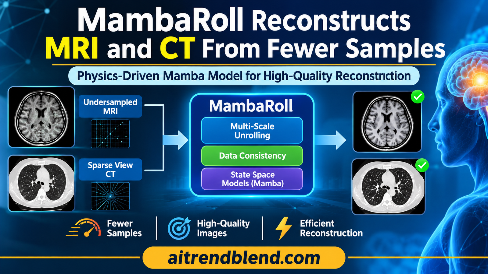
A patient slides into an MRI scanner for a brain exam with three contrasts. Every line of k space the scanner collects costs time, and time in the bore means discomfort, motion and a longer waiting list. Down the corridor, a lung CT faces a similar bargain, where fewer projection views would mean less radiation but more streaks in the image. Both problems ask the same question. How much of the picture can software recover from measurements that were never taken?
A group at Bilkent University in Ankara, led by Tolga Çukur, offers an answer built on state space models, the family behind Mamba. Their model, MambaRoll, reconstructs brain MRI and lung CT from undersampled data by rebuilding the image coarse to fine, checking it against the scanner physics at every scale. The results are strong. The more interesting story is which parts of the design actually earn them.
Key points
- MambaRoll is an unrolled, physics driven network. Each of its cascades predicts feature maps at three spatial scales in order, each scale conditioned on the coarser ones, with a data consistency step after every scale.
- On fastMRI brain data it averaged 40.91 dB PSNR across 4, 8 and 12 fold acceleration, and on LoDoPaB-CT lung data 38.39 dB across 4 to 8 fold view reduction, the best of every model tested.
- Against the strongest competitor in each table the average margin is about 1.2 dB by our arithmetic, smaller than the 2.82 dB and 2.44 dB the paper reports against an average of two state space baselines.
- The ablation shows data consistency and the compressed SSM blocks matter more than the autoregressive link between scales, which is worth 0.89 dB on MRI and 1.46 dB on CT.
- Inference takes about 30 ms per MRI slice and 50 ms per CT slice in the authors’ setup, fast for its accuracy class, although CT memory is several times that of the lightest state space baseline.
- Evidence is retrospective and two dimensional, CT views are simulated with parallel beam geometry, and image quality was judged by one radiologist on 20 samples per task.
Medical disclaimer. This article explains published research on medical image reconstruction. It is not medical advice, diagnosis or treatment, and it does not evaluate any approved clinical product. Reconstruction software used on patient scans must be validated and supervised by qualified professionals. If you have questions about your own imaging, please talk to your care team.
Why undersampled scans are hard to reconstruct
MRI and CT do not take pictures. An MRI scanner samples the Fourier transform of the anatomy, called k space, one line or point at a time, and a CT scanner records line integrals of tissue attenuation from many angles. The image only exists after a computer inverts those measurements. Collect fewer of them and you save time or dose, but the inversion stops having a unique answer. Zero filling the missing k space produces aliasing, and filtered back projection from a handful of CT views produces streaks that run across the whole field of view.
The textbook way out is to add prior knowledge. The reconstruction becomes an optimization that balances agreement with the measured data against a penalty that prefers plausible anatomy. Deep learning replaced the hand written penalty with a learned one, and the most successful designs keep the physics in the loop. These physics driven networks alternate between a learned denoising step and a data consistency step that pulls the estimate back toward what the scanner actually measured. MoDL from Aggarwal, Mani and Jacob in IEEE Transactions on Medical Imaging in 2019 is the classic example of this unrolled pattern, and it appears among the baselines here.
Forward model and regularized reconstruction
$$ \mathcal{A}x + \varepsilon = y, \qquad \mathcal{A}_{\mathrm{MRI}} = \mathcal{P}\mathcal{F}\mathcal{C}, \qquad \mathcal{A}_{\mathrm{CT}} = \mathcal{R} $$ $$ \hat{x} = \arg\min_{x} \; \lVert \mathcal{A}x – y \rVert_2^2 + R(x) $$\(\mathcal{P}\) is the k space sampling pattern, \(\mathcal{F}\) the Fourier transform, \(\mathcal{C}\) the coil sensitivities and \(\mathcal{R}\) the Radon transform. \(R(x)\) is the image prior, which the network learns.
Unrolling turns that optimization into a fixed number of network stages, called cascades. Each cascade takes the previous estimate, runs it through a learned module, and then applies a closed form data consistency correction.
One cascade of an unrolled network
$$ \hat{x}_k = G_{\theta_k}\big(\hat{x}_{k-1};\, \mathcal{A}, y\big), \qquad \hat{x}_0 = \mathcal{A}^{\dagger} y $$ $$ \Psi_{dc}(v_{in}; \mathcal{A}, y) = v_{in} + \mathcal{A}^{\dagger}\big(y – \mathcal{A}v_{in}\big) $$\(\mathcal{A}^{\dagger}\) is the Hermitian adjoint. The correction adds back whatever part of the measured data the current estimate fails to explain.
The physics step is the same for every unrolled network. What differs is the learned module, and that is where the paper places its bet.
Where convolutions, transformers and Mamba each fall short
Separating aliasing from anatomy needs context. An aliased copy of the skull can land inside the brain, and a CT streak can cross half the chest, so the network has to compare pixels that sit far apart. Convolutional networks are good at local texture and poor at that kind of long range reasoning. Transformers handle it in principle, but full attention over a 320 by 320 image is expensive, so practical reconstruction transformers restrict attention to windows or lower resolutions and give back some of the context they promised.
State space models are the current attempt to get both. They flatten an image into a one dimensional sequence and pass it through a learned linear dynamical system whose hidden state carries information along the sequence. The cost grows linearly with sequence length rather than quadratically, as it does for attention. Vision Mamba from Zhu and colleagues at ICML 2024 and VMamba from Liu and colleagues at NeurIPS 2024 brought the idea to images, and our article on the TEAMS Mamba snake for organ contours shows how the same machinery has spread into medical segmentation.
Raster scanning has a cost of its own. Two pixels that are neighbors in the image can end up hundreds of positions apart in the sequence, because one sits on the row below the other. Earlier reconstruction models such as the data driven MambaMIR from Huang and colleagues and the physics driven MambaRecon from Korkmaz and Patel at WACV 2025 ran their state space blocks at a single spatial scale. The authors argue that this leaves context on the table, and their effective receptive field maps, discussed below, are meant to show it.
How MambaRoll works
MambaRoll comes from Bilal Kabas, Fuat Arslan, Valiyeh A. Nezhad, Emine U. Saritas and Tolga Çukur in the Department of Electrical and Electronics Engineering at Bilkent University, with Kader K. Oguz of the National Magnetic Resonance Research Center at Bilkent, the University of California Davis and Ankara Haci Bayram Veli University, and Saban Ozturk of the National Magnetic Resonance Research Center. It is published open access in IEEE Transactions on Medical Imaging, volume 45, issue 10, and it began life as an arXiv preprint in December 2024.
The model takes a linear reconstruction as input, zero filled MRI with real and imaginary channels or filtered back projection for CT, and passes it through K cascades. Inside each cascade, three PD-SSM modules work at a quarter, a half and the full image resolution. The coarsest module goes first. Each later module sees the input image plus every coarser output, so the fine scale prediction is conditioned on what the coarse scales already decided. A small refinement module of two convolutions then restores fine texture and produces the cascade’s output.
Autoregressive prediction across scales
$$ f_s = \mathrm{PD\text{-}SSM}_s\big(f_{\lt s}\big), \qquad f_{\lt s} = [f_0\; f_1\; \dots\; f_{s-1}], \quad s \in \{1, \dots, S\} $$ $$ \hat{x}_k = \mathrm{RM}(f_S) = \mathrm{Conv}\big(\sigma(\mathrm{Conv}(f_S))\big) $$\(f_0 = \hat{x}_{k-1}\), the previous estimate. Every \(f_s\) lives on the full image grid, and each PD-SSM module changes resolution internally.
The borrowing here is explicit. The authors cite visual autoregressive modeling, VAR, from Tian and colleagues at NeurIPS 2024, which generates images by predicting the next scale rather than the next pixel. MambaRoll applies the same coarse to fine logic to reconstruction, with one important difference. Every scale is tied back to the measured data.
Inside one PD-SSM module
Each module does four things. A convolutional encoder maps its input down to the module’s scale, and coarser scales get more channels, with expansion factors of 4, 2 and 1. A compressed SSM block then models long range structure. A convolutional decoder brings the result back to full resolution as an image estimate. Finally a residual data consistency block corrects that estimate against the measurements and passes both versions forward.
Encoder at scale s
$$ d_s = \mathrm{Enc}_s(f_{\lt s}) = \sigma\big(\mathrm{Conv}_{\mathrm{down}}(\sigma(\mathrm{Conv}(f_{\lt s})))\big), \qquad d_s \in \mathbb{R}^{H_s \times W_s \times C_s} $$ $$ H_s = H / 2^{S-s}, \qquad W_s = W / 2^{S-s}, \qquad C_s = 2^{S-s} C $$The compressed SSM block is where the efficiency comes from. A sequence model’s cost depends on sequence length, so the block first rearranges each 4 by 4 neighborhood of the feature map into the channel dimension, a space to depth operation with a factor \(J = 4\). That shortens the sequence by a factor of 16 and multiplies the channels by 16. A sweep scan turns the map into a sequence, a state space layer with a state dimension of 16 processes every channel independently, and a depth to space operation restores the spatial layout before a residual connection adds the input back.
The state space recurrence
$$ h_s[n, c] = \mathbf{A}\, h_s[n-1, c] + \mathbf{B}\, z_s[n, c], \qquad \bar{z}_s[n, c] = \mathbf{C}\, h_s[n, c] $$ $$ g_s = \bar{d}_s + d_s $$\(z_s\) is the compressed sequence of length \(H_s W_s / J^2\), \(h_s\) a hidden state of dimension \(D = 16\), and \(\bar{d}_s\) the restored map after depth to space.
Think of it as reading a page in blocks rather than letters. Each element of the sequence now stands for a small patch, so two regions that were far apart in a pixel raster sit much closer together, and the hidden state has fewer steps over which to forget.
Data consistency at every scale
After decoding, each module produces a full resolution image estimate \(u_s\), corrects it with the same closed form data consistency step used between cascades, and concatenates the raw and corrected versions. Concatenation is a deliberate choice. Replacing \(u_s\) with its corrected version would force the physics on every layer at full strength. Passing both lets later layers decide how much to trust the correction, which the authors argue helps when the imaging operator is imperfect.
Decoder and residual data consistency
$$ u_s = \mathrm{Dec}_s(g_s) = \mathrm{Conv}\big(\sigma(\mathrm{Conv}_{\mathrm{up}}(g_s))\big) $$ $$ \tilde{u}_s = u_s + \mathcal{A}^{\dagger}\big(y – \mathcal{A}u_s\big), \qquad f_s = [u_s \;\; \tilde{u}_s] $$Supervising every scale with the DMSD loss
Multi scale networks often supervise only the final output and hope the intermediate scales learn something useful. MambaRoll adds a deep multi scale decoding loss, DMSD, at the last cascade. The feature map at each scale is decoded to a full resolution image with the module’s own decoder, passed through data consistency, and compared with the ground truth. Because the decoders are shared, the loss adds no new parameters. The authors used a fixed weight of one and did not tune it.
DMSD and total loss
$$ \mathcal{L}_{\mathrm{DMSD}} = \sum_{s=1}^{S} \big\lVert \tilde{u}_s^{K} – x_K \big\rVert_1 = \sum_{s=1}^{S} \big\lVert \mathrm{DC}\big(\mathrm{Dec}_s(g_s^{K})\big) – x_K \big\rVert_1 $$ $$ \mathcal{L}_{\mathrm{total}} = \lVert \hat{x}_K – x_K \rVert_1 + \mathcal{L}_{\mathrm{DMSD}} $$Key takeaway
MambaRoll stacks four ideas, an unrolled physics loop, multi scale state space modeling, coarse to fine autoregressive conditioning and supervision at every scale. The name highlights the autoregression, but as the ablation shows, it is not the part doing most of the work.
How the experiments were set up
For MRI the authors used multi coil brain data from fastMRI with T1, T2 and FLAIR contrasts. Each volume contributed ten cross sections of 320 by 320 pixels, coils were compressed to five virtual coils that preserve 90 percent of the variance, and sensitivities were estimated with ESPIRiT. The split was 240, 60 and 120 subjects for training, validation and test, which across three contrasts gives 7200, 1800 and 3600 cross sections. Undersampling at 4, 8 and 12 fold used two dimensional variable density patterns drawn from a Gaussian density.
For CT they used lung data from LoDoPaB-CT, with 90 cross sections of 352 by 352 pixels per volume and a split of 30, 6 and 12 subjects, giving 2700, 540 and 1080 cross sections. Ground truth reconstructions were Radon transformed with two dimensional parallel beam geometry, and the sinograms were thinned uniformly across angles at 4, 6 and 8 fold. Filtered back projection supplied the linear starting point.
The baselines span every family. For MRI they include the convolutional UNet and MoDL, the transformers SwinMR, SSDiffRecon and DSFormer, and the state space models MambaMIR and MambaRecon. For CT they include FBPConvNet and MetaInv-Net, the transformers USwin, SSDiffRecon and RegFormer, and the state space models MambaMIR and a physics driven PD-Mamba built on VMamba. Every baseline was retrained by the authors with an L1 loss, with the number of cascades and the learning rate tuned per method on validation data. Five cascades were near optimal for MRI and three for CT. Training ran for 50 epochs with Adam on an NVIDIA RTX 4000 Ada GPU, on two dimensional cross sections, and differences were tested with Wilcoxon signed rank tests.
What the numbers show
| Model | Type | R = 4 | R = 8 | R = 12 | Average PSNR | Average SSIM |
|---|---|---|---|---|---|---|
| UNet | CNN, data driven | 36.25 | 33.93 | 30.29 | 33.49 | 91.84 |
| MoDL | CNN, physics driven | 41.76 | 37.56 | 35.87 | 38.39 | 95.28 |
| SwinMR | Transformer, data driven | 37.31 | 34.10 | 32.60 | 34.67 | 91.95 |
| SSDiffRecon | Transformer, physics driven | 42.47 | 37.99 | 35.95 | 38.80 | 95.18 |
| DSFormer | Transformer, physics driven | 43.13 | 38.69 | 36.90 | 39.57 | 95.39 |
| MambaMIR | SSM, data driven | 38.58 | 36.05 | 34.70 | 36.44 | 93.05 |
| MambaRecon | SSM, physics driven | 43.45 | 38.74 | 37.03 | 39.74 | 95.91 |
| MambaRoll | SSM, physics driven | 45.55 | 39.51 | 37.68 | 40.91 | 96.43 |
MambaRoll tops every column, and the authors report that its advantage over each competitor is significant at p below 0.05. Averaged across the three acceleration rates it reaches 40.91 dB and 96.43 percent SSIM. Physics driven models beat their data driven cousins across the board, which is the most consistent pattern in the table. MoDL, a convolutional network with a physics loop, outscores the data driven transformer SwinMR by almost 4 dB on average.
| Model | Type | R = 4 | R = 6 | R = 8 | Average PSNR | Average SSIM |
|---|---|---|---|---|---|---|
| FBPConvNet | CNN, data driven | 34.41 | 33.85 | 32.49 | 33.58 | 84.10 |
| MetaInv-Net | CNN, physics driven | 36.31 | 33.10 | 31.17 | 33.53 | 85.25 |
| USwin | Transformer, data driven | 36.41 | 33.48 | 32.11 | 34.00 | 87.86 |
| SSDiffRecon | Transformer, physics driven | 38.25 | 34.92 | 31.40 | 34.86 | 86.64 |
| RegFormer | Transformer, physics driven | 39.88 | 36.85 | 34.79 | 37.17 | 89.70 |
| MambaMIR | SSM, data driven | 37.42 | 35.42 | 33.92 | 35.59 | 86.68 |
| PD-Mamba | SSM, physics driven | 38.99 | 35.90 | 34.06 | 36.32 | 88.75 |
| MambaRoll | SSM, physics driven | 40.72 | 38.00 | 36.44 | 38.39 | 91.42 |
On CT the picture is similar, with an average of 38.39 dB and 91.42 percent SSIM, and the authors again report significance against every baseline. The gap to convolutional models is wider here than for MRI, which the authors attribute to streaks that span long distances and defeat models built around local filters.
How big is the margin, really?
The paper summarizes MambaRoll’s gains over state space baselines as 2.82 dB in MRI and 2.44 dB in CT. Those figures are averages over the two state space baselines in each table, and one of them in each case is a weaker data driven model. Against the strongest competitor, the picture is more modest. By our arithmetic from Tables I and II, MambaRoll leads MambaRecon by 1.17 dB on average in MRI and RegFormer by 1.22 dB in CT.
The margins also move in opposite directions as the task gets harder. In MRI, the lead over MambaRecon is 2.10 dB at 4 fold acceleration, 0.77 dB at 8 fold and 0.65 dB at 12 fold. In CT, the lead over RegFormer grows from 0.84 dB at 4 fold to 1.15 dB at 6 fold and 1.65 dB at 8 fold. If long range context were the whole story, you might expect the MRI advantage to grow with acceleration, as it does in CT, because aliasing becomes more severe. It shrinks instead. The paper does not discuss this pattern, and we can only speculate that at 12 fold every model is limited by missing information rather than by context.
Per slice variability is large too. MambaRoll’s standard deviation at 4 fold MRI is 3.71 dB, wider than its 2.10 dB lead over MambaRecon at that rate. That does not undercut the result, because the Wilcoxon tests are paired and compare models on the same slices, but it does mean the gain is a shift in the average, not a guarantee on any given image.
Key takeaway
MambaRoll is the best model in both tables, by about 1.2 dB over the strongest rival on average. That is a solid gain in reconstruction terms, but it is roughly half the size of the headline figure, which averages over a weaker baseline.
Generalization under shifts
Two shift experiments probe robustness. In the first, models trained at one rate were tested at a harsher one, 8 fold training and 12 fold testing for MRI, 6 fold training and 8 fold testing for CT. In the second, models were trained only on healthy subjects and tested only on patients, using fastMRI+ brain scans with annotated abnormalities at 4 fold and LIDC-IDRI lung scans with nodules at 6 fold. MambaRoll led in all four settings, with significance at p below 0.05.
| Setting | MambaRoll | Strongest rival |
|---|---|---|
| MRI, trained at R = 8, tested at R = 12 | 35.93 (92.68) | MambaRecon 35.45 (91.99) |
| CT, trained at R = 6, tested at R = 8 | 34.68 (85.81) | RegFormer 33.90 (85.03) |
| MRI, healthy to patients, fastMRI+ at R = 4 | 43.51 (98.21) | MambaRecon 41.43 (97.57) |
| CT, healthy to patients, LIDC-IDRI at R = 6 | 38.54 (92.86) | RegFormer 37.56 (91.50) |
The rate shift deserves a second look. Comparing Table III with Table II, MambaRoll trained at 6 fold and tested at 8 fold CT scores 34.68 dB, which is 1.76 dB below the same model trained at 8 fold. RegFormer loses only 0.89 dB in the same comparison. So MambaRoll is still ahead under the shift, but it gives back more of its advantage than its closest rival does. On MRI the drops are similar, 1.75 dB for MambaRoll and 1.58 dB for MambaRecon. These are our comparisons across tables, not analyses the paper reports.
Table IV has one oddity worth flagging. On fastMRI+ at 4 fold, UNet and MambaMIR post SSIM values near 77 to 78 percent while their PSNR is in the mid thirties, and other models sit above 94 percent. The paper does not comment on this, and readers comparing against these baselines may want to check it.
What a radiologist saw
A board certified radiologist with more than 25 years of experience scored 20 randomly selected reconstructions per task on a five point scale, blinded to the method, for 12 fold MRI and 8 fold CT. MambaRoll scored highest in both, by 0.20 points over the next best method for MRI and 0.65 points for CT, with significance at p below 0.05. The reader’s notes describe subtle differences in tissue to fluid boundaries along the ventricular walls and cortical sulci for MRI, and more pronounced differences in lung parenchyma and in streaking across the hilar and mediastinal regions for CT.
This is useful evidence that the PSNR gains are visible, and the authors are frank about its scope.
“future studies with multiple readers and larger cohorts are warranted”
Kabas and colleagues, on their single reader observer study
Does it really see further?
To test the context argument directly, the authors computed effective receptive fields, the gradient of the central output pixel with respect to every input pixel, averaged over test samples and normalized. MambaRoll shows the broadest and most even maps. Conventional state space baselines show crosses along the horizontal and vertical lines that raster scanning favors, windowed transformers show compact patches despite their theoretical global reach, and shallow convolutional models stay tightly local. The authors stress that these maps show the spatial spread of influence rather than absolute strength, which makes them a reasonable proxy for context but not a direct measure of reconstruction quality. Our piece on ScopeMamba YOLO and receptive fields in small object detection covers the same raster bias from the detection side.
Speed and memory
| MRI model | ms | MB | CT model | ms | MB |
|---|---|---|---|---|---|
| UNet | 11.56 | 550 | FBPConvNet | 13.23 | 974 |
| MoDL | 14.99 | 304 | MetaInvNet | 29.16 | 3288 |
| SwinMR | 49.85 | 870 | USwin | 80.59 | 1082 |
| SSDiffRecon | 339.40 | 740 | SSDiffRecon | 346.74 | 3866 |
| DSFormer | 248.89 | 1338 | RegFormer | 48.20 | 5884 |
| MambaMIR | 36.84 | 474 | MambaMIR | 41.29 | 532 |
| MambaRecon | 36.55 | 462 | PD-Mamba | 90.93 | 4244 |
| MambaRoll | 29.67 | 358 | MambaRoll | 49.79 | 3374 |
For MRI, MambaRoll is the fastest of the state space and transformer models at 29.67 ms per slice and uses the least memory of them at 358 MB, close to convolutional efficiency while beating every model on accuracy. That is a strong result, and it suggests the space to depth compression is doing real work.
CT is less clear cut. Every physics driven CT model pays for repeated Radon transforms in its data consistency steps, and MambaRoll’s 3374 MB at inference is about six times the 532 MB of the data driven MambaMIR by our arithmetic, though well below RegFormer’s 5884 MB and PD-Mamba’s 4244 MB. MambaMIR at 41.29 ms and RegFormer at 48.20 ms are also slightly faster. The authors describe the CT result as a favorable trade off between efficiency and performance, which is fair, as long as readers know which model they are trading against.
What the ablations reveal
The ablation table is the most informative part of the paper, and it tells a different story from the title. The authors removed one component at a time and retrained, testing on FLAIR MRI at 4 fold and CT at 4 fold.
| Variant | MRI, FLAIR R = 4 | Drop | CT, R = 4 | Drop |
|---|---|---|---|---|
| MambaRoll | 43.86 (98.43) | 40.72 (94.05) | ||
| Without PD-SSM modules | 40.49 (97.08) | 3.37 | 31.00 (83.50) | 9.72 |
| Without autoregression | 42.97 (98.10) | 0.89 | 39.26 (92.86) | 1.46 |
| Single scale, S = 1 | 42.62 (98.01) | 1.24 | 37.11 (90.53) | 3.61 |
| Without compressed SSM | 41.43 (97.44) | 2.43 | 35.65 (88.51) | 5.07 |
| Without data consistency | 36.88 (93.44) | 6.98 | 38.66 (92.14) | 2.06 |
Removing the autoregressive link, so that each scale sees only the input image and the scales are merged by a learned fusion layer, costs 0.89 dB on MRI and 1.46 dB on CT. That is a real effect, and it is the smallest in the table. Dropping to a single scale costs more, and removing the compressed SSM blocks costs more still, 2.43 dB on MRI and 5.07 dB on CT. Everything in the design helps, but the multi scale state space machinery carries more weight than the conditioning between scales.
The data consistency result is the most striking line. Without it, MRI loses 6.98 dB, by far its largest drop. CT loses only 2.06 dB, while removing the PD-SSM modules costs CT 9.72 dB. In plain terms, MRI reconstruction here leans on physics and CT reconstruction leans on the learned prior. The paper does not interpret this asymmetry. Our reading is that the MRI operator, built from orthonormal Fourier transforms, gives a well conditioned correction, while the adjoint of a sparse Radon transform is an unfiltered back projection that smears corrections across the image, so a single unit step does less. That is a hypothesis, and it would be worth testing with a filtered or scaled correction for CT.
Two design sweeps round this out. Accuracy rose with the number of scales up to three and then flattened, so S of 3 is the efficient choice. For the compression factor, values beyond 4 degraded accuracy without saving time, which the authors attribute to scattering local spatial structure too widely across channels. The DMSD loss also beat three alternatives, single scale supervision, supervision on downsampled outputs and supervision on latent features, on both modalities.
Key takeaway
If you only remember one row, remember data consistency. It is worth almost 7 dB on MRI. The autoregressive idea in the title is worth under 1 dB there, a useful refinement on top of a design whose foundations are physics and compressed state space blocks.
Clinical translation gap
How far is this from a scanner console? Further than the tables suggest, for reasons the authors largely acknowledge.
The undersampling is retrospective. MRI acceleration was simulated by discarding k space from fully sampled scans, and CT sparse views were simulated by Radon transforming reconstructed images with parallel beam geometry. Real accelerated acquisitions carry their own artifacts, and the authors note that clinical CT uses fan beam or helical geometry with photon counting noise that depends on dose, none of which was modeled. Simulating sinograms from images also means the forward model used for training and testing matches the data perfectly, an easier setting than any real scanner provides.
Everything runs on two dimensional cross sections. Clinical MRI and CT are volumetric, and through plane consistency matters for reading and for downstream measurements. The authors list 2.5D processing, small 3D patches and volumetric scan orders as future work.
Each model handles one contrast or one CT protocol at a time. A clinical brain protocol acquires several contrasts in one session, and the authors suggest joint multi contrast reconstruction as an extension. Our article on guided multi contrast reconstruction with SGF MRI shows what that direction can look like.
Training needs fully sampled references. The setup is supervised, and fully sampled data are expensive or impossible to collect in some applications. The authors point to self supervised training and test time adaptation as alternatives.
The reader study is small. One radiologist, 20 samples per task, and score gaps of 0.20 points in MRI are evidence of a visible difference, not of diagnostic equivalence or superiority.
Regulatory and safety note, our reading
Software that reconstructs diagnostic images from undersampled data is regulated as a medical device in most jurisdictions, and learned reconstruction raises a specific safety question, whether it can invent or erase small structures such as lesions. PSNR, SSIM and a single reader study do not answer that question. Any clinical path would need prospective accelerated acquisitions, multi reader diagnostic studies focused on pathology, failure analysis on out of distribution scans, and the usual approval route for the device that wraps the model.
Limitations, sample size and bias
- Modest subject counts. The MRI test set has 120 subjects and the CT test set only 12 subjects, expanded to 3600 and 1080 cross sections. Slices from one subject are correlated, so the Wilcoxon tests over slices likely overstate how independent the evidence is, and the CT result rests on a small number of patients.
- Simulated acquisitions. MRI undersampling is retrospective and CT views are synthesized from reconstructed images with parallel beam geometry and no explicit noise model, which favors every model trained in the same setting.
- Two dimensional only. All results are on single cross sections, and volumetric behavior is untested.
- Dataset bias. fastMRI brain and LoDoPaB-CT lung data come from specific scanners and populations. The cross population tests swap healthy for pathological cases, which is valuable, but they do not test other vendors, field strengths, body regions or pediatric patients.
- Baselines retrained by the authors. Every competitor was retrained with an L1 loss and tuned on validation data, which is a fair protocol. SSDiffRecon was converted from a self supervised to a supervised setup, and MambaRoll alone carries the extra DMSD loss, so the comparison is between full MambaRoll and adapted versions of the others.
- Single reader observer study. One radiologist scored 20 samples per task, which the authors themselves call limited.
- Metrics. PSNR and SSIM reward fidelity to the reference image, which in MRI is itself a reconstruction from fully sampled data. Neither measures whether small lesions are preserved.
What practitioners can take from this
If you build reconstruction networks, the clearest lesson is to measure the physics. MambaRoll’s ablation shows data consistency carrying most of the MRI result, and a well designed correction step may matter more than the backbone you put between corrections. The second lesson is that state space models become practical at full resolution once you compress the sequence. The space to depth trick with J of 4 is simple, it cut sequence length by 16, and the paper’s sweeps suggest it is close to the sweet spot.
If you compare models, report margins against the strongest baseline as well as against an average, and look at how margins change with acceleration. A method that leads by 2 dB at 4 fold and 0.65 dB at 12 fold is telling you something about where its advantage comes from.
The ideas also travel. Coarse to fine prediction with consistency checks at every scale could apply to any inverse problem with a known forward model, from seismic imaging to microscopy deblurring. For a related view of physics as supervision, our article on quantitative T1 and T2 maps from routine brain MRI uses a forward model of the scanner in a very different way. For recovering motion directly from raw MRI data, see our piece on LAPANet and k space cardiac motion estimation. More studies of this kind sit in our Medical AI section.
Conclusion
MambaRoll is a well engineered reconstruction model that wins clearly on both accelerated brain MRI and sparse view lung CT. It averages 40.91 dB across 4 to 12 fold MRI and 38.39 dB across 4 to 8 fold CT, leads every convolutional, transformer and state space baseline the authors tested, holds its lead under shifts in acceleration and patient population, and runs a brain MRI slice in under 30 ms. The code is public, which makes all of this checkable.
The conceptual contribution is the combination of multi scale state space modeling with an unrolled physics loop and coarse to fine conditioning. Each scale makes a prediction, checks it against the measurements and hands it on. The effective receptive field maps support the claim that this captures broader context than single scale state space models, which scan pixels in long rasters and favor the horizontal and vertical directions.
The ablations sharpen what that contribution means. The autoregressive link between scales is the smallest contributor, under 1 dB on MRI, while data consistency and the compressed state space blocks deliver most of the gain. That is not a criticism of the design, because the parts work together, but it should shape how others borrow from it. If you take one idea from MambaRoll, compress your sequences and keep the physics close.
The remaining limits are familiar for reconstruction research. Acquisitions are simulated, the CT geometry is simpler than any clinical scanner, everything is two dimensional, the test cohorts are modest and the reader study is a single radiologist. The margin over the strongest rival is about 1.2 dB on average, real but smaller than the headline.
The authors name the next steps themselves, self supervised and test time training, generative losses, multi contrast reconstruction, realistic CT geometry and volumetric processing. A prospective test on accelerated scans from a different vendor, read by several radiologists with attention to small lesions, would be the most convincing evidence of all.
Undersampling will always throw information away. The best a model can do is reason carefully about what is left, and MambaRoll shows that checking the answer against the physics at every scale is a good way to do it.
A reference implementation in PyTorch
The authors’ code is public at the MambaRoll repository on GitHub, and that is the version to use for any real comparison. The listing below is our own editorial reconstruction from the paper, written to make the architecture easy to read. It implements multi coil MRI and sparse view CT operators with exact adjoints, the data consistency step, the compressed SSM block with space to depth and a sweep scan, PD-SSM modules, autoregressive cascades, the refinement module, the unrolled model, the DMSD and total losses, PSNR and SSIM, a training loop and a smoke test.
Three simplifications are stated in the file header. The state space layer uses a diagonal stable state matrix evaluated as a causal convolution, the sweep scan is a forward and reversed raster over rows, and the CT operator is normalized to unit spectral norm so the unit correction step is stable, a choice the paper does not specify. On random ellipse phantoms at 64 by 64 pixels, with two cascades and a few hundred training steps on a CPU, the toy model raised SSIM from 0.677 to 0.863 over zero filling for 4 fold MRI and PSNR from 19.91 to 22.70 dB over filtered back projection for 4 fold sparse view CT. These numbers only show that the pipeline trains. They say nothing about real anatomy and should not be compared with the paper.
"""
MambaRoll reference sketch in PyTorch
=====================================
An editorial reconstruction of the architecture described in
Kabas, Arslan, Nezhad, Oguz, Ozturk, Saritas and Cukur,
"Physics-Driven Autoregressive State Space Models for Medical Image
Reconstruction", IEEE Transactions on Medical Imaging 45(10), 2026,
DOI 10.1109/TMI.2026.3716153. This is NOT the authors' code. Their
implementation is public at github.com/icon-lab/MambaRoll.

What is here
  * Imaging operators A and their adjoints
      - multi coil Cartesian MRI, A = P F C                             Eq. 1
      - sparse view parallel beam CT as an explicit sparse Radon matrix
  * Data consistency v + A^H (y - A v)                                   Eq. 5, 13
  * Compressed SSM block: space to depth (J), sweep scan, LTI state
    space layer per channel, depth to space, residual                    Eq. 9-11
  * PD-SSM module: encoder, compressed SSM, decoder, residual DC          Eq. 8, 12-14
  * Autoregressive cascade over S scales plus refinement module          Eq. 6-7
  * Unrolled MambaRoll with K cascades, x0 = A^H y (ZF) or FBP           Eq. 3
  * Deep multi scale decoding (DMSD) loss and total loss                  Eq. 15-16
  * Training loop, PSNR / SSIM evaluation, CPU smoke test (about 90 s)

Simplifications, stated plainly
  * The SSM layer uses a diagonal, stable state matrix (S4D style) and
    evaluates the recurrence as a causal convolution with an FFT. The
    paper writes a general A in R^{DxD}; its released code uses Mamba.
  * The sweep scan is a forward plus reversed raster over rows.
  * The CT operator is normalised to unit spectral norm so the unit step
    in Eq. 13 is stable. The paper does not state its operator scaling.
"""
import math
import torch
import torch.nn as nn
import torch.nn.functional as F


# ---------------------------------------------------------------------------
# 1. Imaging operators
# ---------------------------------------------------------------------------
def to_complex(x):            # (B,2,H,W) real/imag -> (B,H,W) complex
    return torch.complex(x[:, 0], x[:, 1])


def to_channels(z):           # (B,H,W) complex -> (B,2,H,W)
    return torch.stack([z.real, z.imag], dim=1)


class MRIOperator:
    """A = P F C for multi coil Cartesian MRI with orthonormal FFTs.
    mask (H,W) in {0,1}, sens (Nc,H,W) complex with sum |C|^2 = 1."""

    def __init__(self, mask, sens):
        self.mask, self.sens = mask, sens
        self.img_ch = 2

    def A(self, x):                              # (B,2,H,W) -> (B,Nc,H,W) complex
        coil = to_complex(x)[:, None] * self.sens[None]
        return torch.fft.fft2(coil, norm="ortho") * self.mask

    def AH(self, y):                             # (B,Nc,H,W) -> (B,2,H,W)
        coil = torch.fft.ifft2(y * self.mask, norm="ortho")
        return to_channels((coil * self.sens.conj()[None]).sum(1))

    def linear_recon(self, y):                   # zero filled reconstruction
        return self.AH(y)


def radon_matrix(n, angles, oversample=1.0):
    """Explicit sparse parallel beam projector for an n x n image on [-1,1]^2.
    Each ray is sampled at n*oversample points with bilinear weights, so the
    adjoint is exactly the transpose."""
    n_t = int(n * oversample)
    th = torch.as_tensor(angles, dtype=torch.float32)
    u = torch.linspace(-1, 1, n)                 # detector bins
    t = torch.linspace(-1, 1, n_t)               # samples along the ray
    T, U, TT = torch.meshgrid(th, u, t, indexing="ij")
    xs = U * torch.cos(T) - TT * torch.sin(T)
    ys = U * torch.sin(T) + TT * torch.cos(T)
    px, py = (xs + 1) * (n - 1) / 2, (ys + 1) * (n - 1) / 2
    x0, y0 = px.floor(), py.floor()
    row = (torch.arange(len(th))[:, None, None] * n + torch.arange(n)[None, :, None]).expand_as(px)
    rows, cols, vals = [], [], []
    for dx in (0, 1):
        for dy in (0, 1):
            xi, yi = x0 + dx, y0 + dy
            w = (1 - (px - xi).abs()) * (1 - (py - yi).abs())
            ok = (xi >= 0) & (xi < n) & (yi >= 0) & (yi < n) & (w > 0)
            rows.append(row[ok]); cols.append((yi[ok] * n + xi[ok]).long()); vals.append(w[ok])
    idx = torch.stack([torch.cat(rows), torch.cat(cols)])
    M = torch.sparse_coo_tensor(idx, torch.cat(vals) * (2.0 / n_t), (len(th) * n, n * n),
                                check_invariants=False)
    return M.coalesce()


class CTOperator:
    """Sparse view CT. A x = R x with R a sparse Radon matrix normalised to
    unit spectral norm. A^H is R^T. linear_recon is a ramp filtered
    backprojection used as the FBP initialisation."""

    def __init__(self, n, angles):
        self.n, self.n_ang = n, len(angles)
        R = radon_matrix(n, angles)
        self.scale = self._spectral_norm(R)
        self.R = (R * (1.0 / self.scale)).coalesce()
        self.Rt = self.R.t().coalesce()
        self.img_ch = 1
        freqs = torch.fft.fftfreq(2 * n)
        self.ramp = 2 * freqs.abs()

    @staticmethod
    def _spectral_norm(R, iters=30):
        v = torch.randn(R.shape[1], 1)
        for _ in range(iters):
            v = torch.sparse.mm(R.t(), torch.sparse.mm(R, v))
            v = v / v.norm()
        return torch.sparse.mm(R, v).norm().item()

    def A(self, x):                              # (B,1,n,n) -> (B,n_ang,n)
        B = x.shape[0]
        flat = x.reshape(B, -1).T
        return torch.sparse.mm(self.R, flat).T.reshape(B, self.n_ang, self.n)

    def AH(self, y):                             # (B,n_ang,n) -> (B,1,n,n)
        B = y.shape[0]
        flat = y.reshape(B, -1).T
        return torch.sparse.mm(self.Rt, flat).T.reshape(B, 1, self.n, self.n)

    def linear_recon(self, y):                   # FBP with a ramp filter
        Y = torch.fft.fft(F.pad(y, (0, self.n)), dim=-1) * self.ramp
        yf = torch.fft.ifft(Y, dim=-1).real[..., :self.n]
        # continuous FBP weights: d(theta) = pi / n_ang, ramp |nu| with detector
        # spacing 2 / (n - 1), and the bilinear backprojector's 2 / n pixel weight
        w = math.pi * self.n / (2 * self.n_ang) * (self.n - 1) / 4
        return self.AH(yf) * w * self.scale ** 2


def data_consistency(v, op, y):
    """Eq. 5 and Eq. 13, a closed form correction with no inner iterations."""
    return v + op.AH(y - op.A(v))


# ---------------------------------------------------------------------------
# 2. Compressed state space block (Eq. 9 to 11)
# ---------------------------------------------------------------------------
class DiagonalSSM(nn.Module):
    """h[n] = A h[n-1] + B z[n],  zbar[n] = C h[n], per channel, with a
    diagonal A = exp(dt * a), a < 0 (zero order hold). Runs as a causal
    convolution with kernel K[n] = C diag(A^n) B, computed by FFT."""

    def __init__(self, channels, d_state=16):
        super().__init__()
        self.log_dt = nn.Parameter(torch.empty(channels).uniform_(math.log(1e-3), math.log(1e-1)))
        self.log_a = nn.Parameter(torch.log(0.5 + torch.arange(d_state).float()).repeat(channels, 1))
        self.B = nn.Parameter(torch.randn(channels, d_state) / math.sqrt(d_state))
        self.C = nn.Parameter(torch.randn(channels, d_state) / math.sqrt(d_state))
        self.Dskip = nn.Parameter(torch.ones(channels))

    def kernel(self, L):
        dt = self.log_dt.exp()[:, None]                       # (ch,1)
        a = -self.log_a.exp()                                 # (ch,D) stable poles
        dA = torch.exp(dt * a)                                # (ch,D)
        dB = (dA - 1.0) / a * self.B                          # ZOH discretisation
        n = torch.arange(L, device=a.device, dtype=a.dtype)
        powers = torch.exp((dt * a)[..., None] * n)           # (ch,D,L)
        return torch.einsum("cd,cdl->cl", self.C * dB, powers)

    def forward(self, z):                                     # z (B,ch,L)
        L = z.shape[-1]
        K = self.kernel(L)
        Zf = torch.fft.rfft(z, n=2 * L)
        Kf = torch.fft.rfft(K, n=2 * L)
        y = torch.fft.irfft(Zf * Kf[None], n=2 * L)[..., :L]
        return y + self.Dskip[None, :, None] * z


class CompressedSSM(nn.Module):
    """Space to depth by J shortens the sequence by J^2, a sweep scan turns
    the map into a sequence, the SSM runs per channel, then depth to space
    restores resolution and the result is added back (Eq. 11)."""

    def __init__(self, channels, J=4, d_state=16):
        super().__init__()
        self.J = J
        self.norm = nn.GroupNorm(1, channels * J * J)
        self.ssm = DiagonalSSM(channels * J * J, d_state)

    def forward(self, d):                                     # d (B,C,H,W)
        B, C, H, W = d.shape
        J = self.J if (H % self.J == 0 and W % self.J == 0) else 1
        x = F.pixel_unshuffle(d, J) if J > 1 else d            # (B, C J^2, H/J, W/J)
        x = self.norm(x) if J == self.J else x
        h, w = x.shape[-2:]
        seq = x.flatten(2)                                    # row raster sweep
        if J == self.J:
            out = self.ssm(seq) + self.ssm(seq.flip(-1)).flip(-1)
        else:                                                  # tiny maps fall back to identity
            out = seq
        out = out.reshape(B, -1, h, w)
        dbar = F.pixel_shuffle(out, J) if J > 1 else out
        return dbar + d                                       # g_s = dbar_s + d_s


# ---------------------------------------------------------------------------
# 3. PD-SSM module and one cascade (Eq. 6 to 8, 12 to 14)
# ---------------------------------------------------------------------------
class PDSSM(nn.Module):
    """Scale s of S. Encodes f_<s down to (H/2^(S-s), W/2^(S-s)) with
    2^(S-s) C channels, applies the compressed SSM, decodes back to the
    image grid, enforces data consistency and concatenates [u, DC(u)]."""

    def __init__(self, in_ch, img_ch, C, s, S, J=4, d_state=16):
        super().__init__()
        self.factor = 2 ** (S - s)
        Cs = C * self.factor
        self.enc = nn.Sequential(
            nn.Conv2d(in_ch, C, 3, padding=1), nn.SiLU(),
            nn.Conv2d(C, Cs, 3, stride=self.factor, padding=1) if self.factor > 1
            else nn.Conv2d(C, Cs, 3, padding=1),
            nn.SiLU())
        self.ssm = CompressedSSM(Cs, J, d_state)
        up = (nn.ConvTranspose2d(Cs, C, self.factor, stride=self.factor) if self.factor > 1
              else nn.Conv2d(Cs, C, 3, padding=1))
        self.dec = nn.Sequential(up, nn.SiLU(), nn.Conv2d(C, img_ch, 3, padding=1))

    def forward(self, f_lt_s, op, y):
        d = self.enc(f_lt_s)                                  # Eq. 8
        g = self.ssm(d)                                       # Eq. 9 to 11
        u = self.dec(g)                                       # Eq. 12
        u_dc = data_consistency(u, op, y)                     # Eq. 13
        return torch.cat([u, u_dc], dim=1), u_dc              # Eq. 14


class Cascade(nn.Module):
    """Autoregressive prediction across scales. Each PD-SSM sees the input
    and every coarser scale output, f_<s = [f_0, f_1, ..., f_{s-1}]."""

    def __init__(self, img_ch, C=16, S=3, J=4, d_state=16, autoregressive=True):
        super().__init__()
        self.S, self.ar = S, autoregressive
        f_ch = 2 * img_ch                                     # [u, DC(u)]
        self.blocks = nn.ModuleList()
        for s in range(1, S + 1):
            in_ch = img_ch + (s - 1) * f_ch if autoregressive else img_ch
            self.blocks.append(PDSSM(in_ch, img_ch, C, s, S, J, d_state))
        rm_in = f_ch if autoregressive else S * f_ch
        self.refine = nn.Sequential(nn.Conv2d(rm_in, C, 3, padding=1), nn.SiLU(),
                                    nn.Conv2d(C, img_ch, 3, padding=1))   # Eq. 7

    def forward(self, x_prev, op, y):
        feats, u_dcs = [x_prev], []
        for blk in self.blocks:
            inp = torch.cat(feats, dim=1) if self.ar else x_prev
            f_s, u_dc = blk(inp, op, y)
            feats.append(f_s); u_dcs.append(u_dc)
        rm_in = feats[-1] if self.ar else torch.cat(feats[1:], dim=1)
        return self.refine(rm_in), u_dcs


class MambaRoll(nn.Module):
    """K unrolled cascades, x_k = G_k(x_{k-1}; A, y), x_0 = linear recon."""

    def __init__(self, img_ch, K=5, C=16, S=3, J=4, d_state=16, autoregressive=True):
        super().__init__()
        self.cascades = nn.ModuleList(
            [Cascade(img_ch, C, S, J, d_state, autoregressive) for _ in range(K)])

    def forward(self, y, op):
        x = op.linear_recon(y)
        for casc in self.cascades:
            x, u_dcs = casc(x, op, y)
        return x, u_dcs                                       # u_dcs from the last cascade


# ---------------------------------------------------------------------------
# 4. Losses (Eq. 15 and 16)
# ---------------------------------------------------------------------------
def dmsd_loss(u_dcs, target):
    """Sum over scales of || DC(Dec_s(g_s^K)) - x ||_1 at the final cascade.
    The decoders are the ones inside the PD-SSM blocks, so no new weights."""
    return sum(F.l1_loss(u, target) for u in u_dcs)


def total_loss(x_hat, u_dcs, target, use_dmsd=True):
    rec = F.l1_loss(x_hat, target)
    return rec + (dmsd_loss(u_dcs, target) if use_dmsd else 0.0)


# ---------------------------------------------------------------------------
# 5. Metrics
# ---------------------------------------------------------------------------
def magnitude(x):
    return x.norm(dim=1, keepdim=True) if x.shape[1] == 2 else x.abs()


def psnr(x, ref):
    x, ref = magnitude(x), magnitude(ref)
    mse = ((x - ref) ** 2).flatten(1).mean(1)
    peak = ref.flatten(1).amax(1)
    return (10 * torch.log10(peak ** 2 / mse.clamp_min(1e-12))).mean().item()


def ssim(x, ref, win=7):
    x, ref = magnitude(x), magnitude(ref)
    peak = ref.flatten(1).amax(1).view(-1, 1, 1, 1)
    x, ref = x / peak, ref / peak
    g = torch.exp(-((torch.arange(win) - win // 2) ** 2) / (2 * 1.5 ** 2))
    g = (g / g.sum())
    k = (g[:, None] * g[None, :])[None, None]
    mu = lambda t: F.conv2d(t, k, padding=win // 2)
    mx, my = mu(x), mu(ref)
    sx, sy, sxy = mu(x * x) - mx ** 2, mu(ref * ref) - my ** 2, mu(x * ref) - mx * my
    c1, c2 = 0.01 ** 2, 0.03 ** 2
    s = ((2 * mx * my + c1) * (2 * sxy + c2)) / ((mx ** 2 + my ** 2 + c1) * (sx + sy + c2))
    return s.mean().item()


# ---------------------------------------------------------------------------
# 6. Training and evaluation
# ---------------------------------------------------------------------------
def train(model, op_fn, data_fn, steps=200, lr=1e-3, use_dmsd=True, log_every=25):
    """data_fn() returns a clean batch. op_fn() returns an operator, so masks
    or view sets can be resampled. Adam with betas (0.9, 0.999) as in the paper."""
    opt = torch.optim.Adam(model.parameters(), lr=lr, betas=(0.9, 0.999))
    hist = []
    for step in range(1, steps + 1):
        x = data_fn()
        op = op_fn()
        y = op.A(x)
        x_hat, u_dcs = model(y, op)
        loss = total_loss(x_hat, u_dcs, x, use_dmsd)
        opt.zero_grad()
        loss.backward()
        opt.step()
        hist.append(loss.item())
        if step % log_every == 0:
            print(f"    step {step:4d}  loss {sum(hist[-log_every:]) / log_every:.4f}")
    return hist


@torch.no_grad()
def evaluate(model, op, x):
    y = op.A(x)
    x0 = op.linear_recon(y)
    x_hat, _ = model(y, op)
    return {"linear_psnr": psnr(x0, x), "linear_ssim": ssim(x0, x),
            "model_psnr": psnr(x_hat, x), "model_ssim": ssim(x_hat, x)}


# ---------------------------------------------------------------------------
# 7. Synthetic data for the smoke test
# ---------------------------------------------------------------------------
def random_phantoms(B, n, gen):
    """Random ellipse phantoms in [0,1], a stand in for brain or lung slices."""
    yy, xx = torch.meshgrid(torch.linspace(-1, 1, n), torch.linspace(-1, 1, n), indexing="ij")
    out = torch.zeros(B, 1, n, n)
    for b in range(B):
        img = torch.zeros(n, n)
        img += 0.6 * (((xx / 0.85) ** 2 + (yy / 0.95) ** 2) <= 1).float()
        for _ in range(6):
            cx, cy = (torch.rand(2, generator=gen) - 0.5) * 1.0
            ax, ay = 0.08 + 0.3 * torch.rand(2, generator=gen)
            ang = math.pi * torch.rand(1, generator=gen).item()
            xr = (xx - cx) * math.cos(ang) + (yy - cy) * math.sin(ang)
            yr = -(xx - cx) * math.sin(ang) + (yy - cy) * math.cos(ang)
            img += (torch.rand(1, generator=gen).item() - 0.3) * 0.5 * (((xr / ax) ** 2 + (yr / ay) ** 2) <= 1).float()
        out[b, 0] = img.clamp(0, 1)
    return out


def variable_density_mask(n, R, gen, center=0.08):
    """2D variable density pattern from a Gaussian density, fully sampled centre."""
    yy, xx = torch.meshgrid(torch.linspace(-1, 1, n), torch.linspace(-1, 1, n), indexing="ij")
    pdf = torch.exp(-(xx ** 2 + yy ** 2) / (2 * 0.3 ** 2))
    pdf = pdf / pdf.sum() * (n * n / R)
    mask = (torch.rand(n, n, generator=gen) < pdf.clamp(max=1)).float()
    mask[(xx.abs() < center) & (yy.abs() < center)] = 1
    return torch.fft.ifftshift(mask)


def coil_maps(n, nc=4):
    yy, xx = torch.meshgrid(torch.linspace(-1, 1, n), torch.linspace(-1, 1, n), indexing="ij")
    maps = []
    for c in range(nc):
        a = 2 * math.pi * c / nc
        mag = torch.exp(-((xx - 0.9 * math.cos(a)) ** 2 + (yy - 0.9 * math.sin(a)) ** 2) / 1.2)
        maps.append(mag * torch.exp(1j * (a + 0.5 * xx)))
    S = torch.stack(maps)
    return S / torch.sqrt((S.abs() ** 2).sum(0, keepdim=True))


if __name__ == "__main__":
    torch.manual_seed(0)
    torch.set_num_threads(2)
    gen = torch.Generator().manual_seed(0)
    n = 64

    # ---- accelerated MRI, R = 4, four coils, complex images ----
    print("MRI, R = 4, 4 coils")
    sens = coil_maps(n, 4)
    phase = lambda x: torch.cat([x, torch.zeros_like(x)], 1)       # real valued toy images
    mri_data = lambda: phase(random_phantoms(4, n, gen))
    mri_op = lambda: MRIOperator(variable_density_mask(n, 4, gen), sens)
    model = MambaRoll(img_ch=2, K=2, C=12, S=3, J=4, d_state=16)
    print("  parameters", sum(p.numel() for p in model.parameters()))
    hist = train(model, mri_op, mri_data, steps=300, lr=2e-3, log_every=100)
    test_x = phase(random_phantoms(8, n, torch.Generator().manual_seed(123)))
    test_op = MRIOperator(variable_density_mask(n, 4, torch.Generator().manual_seed(7)), sens)
    r_mri = evaluate(model, test_op, test_x)
    print("  test", {k: round(v, 3) for k, v in r_mri.items()})

    # ---- sparse view CT, 60 views reduced to 15 (R = 4) ----
    print("CT, 60 views to 15 views (R = 4)")
    ang = torch.linspace(0, math.pi, 61)[:-1][::4]
    ct = CTOperator(n, ang)
    ct_data = lambda: random_phantoms(4, n, gen)
    model_ct = MambaRoll(img_ch=1, K=2, C=12, S=3, J=4, d_state=16)
    hist_ct = train(model_ct, lambda: ct, ct_data, steps=150, lr=2e-3, log_every=50)
    r_ct = evaluate(model_ct, ct, random_phantoms(8, n, torch.Generator().manual_seed(321)))
    print("  test", {k: round(v, 3) for k, v in r_ct.items()})

    # ---- adjoint check and shape checks ----
    x = torch.randn(2, 1, n, n); yv = torch.randn(2, len(ang), n)
    lhs = (ct.A(x) * yv).sum(); rhs = (x * ct.AH(yv)).sum()
    print("  CT adjoint mismatch", abs(lhs - rhs).item() / abs(lhs).item())
    assert abs(lhs - rhs) / abs(lhs) < 1e-4
    assert hist[-1] < hist[0] and hist_ct[-1] < hist_ct[0]
    print("smoke test passed")
Frequently asked questions
What is MambaRoll?
MambaRoll is a deep learning model for reconstructing medical images from undersampled MRI and sparse view CT data, published in IEEE Transactions on Medical Imaging in 2026 by researchers at Bilkent University. It unrolls a physics driven network into cascades, and each cascade predicts features at three spatial scales with state space model blocks, checking every scale against the measured data.
How accurate is MambaRoll compared with other reconstruction methods?
On fastMRI brain data it averaged 40.91 dB PSNR across 4, 8 and 12 fold acceleration, and on LoDoPaB-CT lung data 38.39 dB across 4 to 8 fold view reduction, ahead of every convolutional, transformer and state space baseline tested. Against the strongest rival in each table the average lead is about 1.2 dB.
What does the autoregressive part of MambaRoll do?
Each cascade predicts feature maps from coarse to fine. The quarter resolution scale goes first, and each finer scale sees the input and every coarser prediction. In the ablation, removing this conditioning cost 0.89 dB on MRI and 1.46 dB on CT, smaller than the losses from removing data consistency or the compressed state space blocks.
Why does data consistency matter so much in MambaRoll?
Data consistency corrects each intermediate image so that it agrees with the measurements the scanner actually collected. Removing it cost MambaRoll 6.98 dB on MRI, its largest single loss, but only 2.06 dB on CT, where the learned state space modules carried more of the result.
Is MambaRoll fast enough for clinical use?
In the authors’ tests it reconstructed an MRI cross section in 29.67 ms using 358 MB of memory, faster than every transformer and state space baseline. For CT it took 49.79 ms and 3374 MB, which is more memory than the data driven MambaMIR but less than other physics driven models.
Can MambaRoll be used on patient scans today?
No. It was evaluated on retrospectively undersampled two dimensional data, with CT views simulated in parallel beam geometry, and judged by one radiologist on 20 samples per task. It has no regulatory clearance, and clinical use would need prospective validation and review by qualified staff.
Read the paper and explore the code
The article is open access under a Creative Commons Attribution license in IEEE Transactions on Medical Imaging, with every table, the effective receptive field maps and the full ablation sweeps. The authors’ PyTorch implementation is public.
Kabas, B., Arslan, F., Nezhad, V. A., Oguz, K. K., Ozturk, S., Saritas, E. U., and Çukur, T. Physics driven autoregressive state space models for medical image reconstruction. IEEE Transactions on Medical Imaging 45(10), October 2026, pages 5153 to 5165. DOI 10.1109/TMI.2026.3716153. Open access under CC BY 4.0. The work was supported in part by TUBA GEBIP 2015 and BAGEP 2017 fellowships and by TUBITAK 1001 grant 121E488.
This analysis is based on the published paper and an independent evaluation of its claims.