
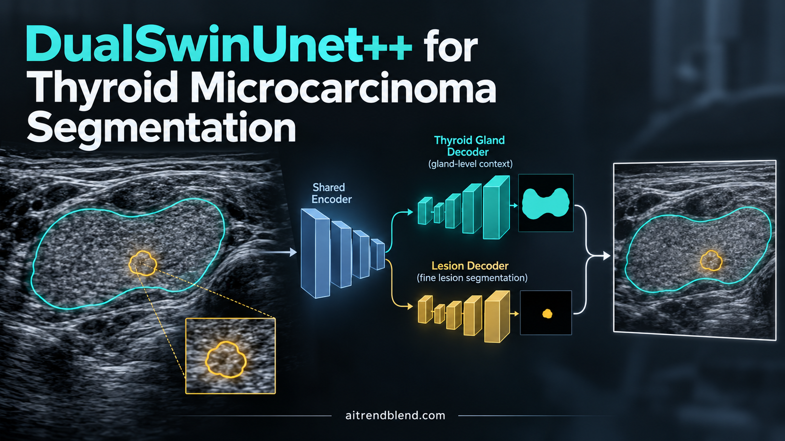
Inside an interventional radiology suite, an awake patient under regional neck anesthesia swallows involuntarily while a clinician guides a high frequency radiofrequency ablation electrode toward a papillary thyroid microcarcinoma measuring less than ten millimeters across. Every burst of alternating electrical current heats the malignant tissue and releases a cloud of microscopic gas bubbles that linger for minutes, casting dense acoustic shadows across the B-mode ultrasound monitor and obscuring the exact tumor margin the physician needs to see next. Maryam Dialameh, Hossein Rajabzadeh, Moslem Sadeghi-Goughari, Jung Suk Sim, and Hyock Ju Kwon at the University of Waterloo and Withsim Clinic in Seongnam designed DualSwinUnet++ to anchor tumor delineation inside the anatomical boundary of the thyroid gland itself, cutting false positive alerts while returning updated segmentation masks in 180 milliseconds.
Key Research Takeaways
- DualSwinUnet++ extends the pure transformer Swin-Unet backbone with two parallel hierarchical decoders that separate macroscopic organ localization (the thyroid gland) from microscopic lesion delineation (papillary thyroid microcarcinoma, or PTMC).
- Rather than sharing a single output projection head, each decoder uses an independent linear projection layer and dedicated hybrid Binary Cross Entropy plus Dice supervision to prevent competing gradient interference.
- Six U-Net style concatenated skip connections (three from the encoder to Decoder 1, and three combining encoder and Decoder 1 features into Decoder 2) outperform additive residual fusion by 6.51 percentage points in Dice on clinical RFA scans.
- Evaluated on 691 clinical RFA ultrasound frames from 101 patients and 3,493 public TN3K thyroid nodule images, DualSwinUnet++ achieves 84.36 percent Dice (71.23 percent Jaccard) on the RFA cohort and 81.24 percent Dice (69.14 percent Jaccard) on TN3K.
- An average inference latency of 0.18 seconds per frame delivers more than five spatial updates per second, outpacing diffusion segmentation models such as SegDiff (0.36 seconds) and Medsegdiff-v2 (0.31 seconds) while scoring 2.49 to 2.68 percentage points higher in Dice.
This article analyzes peer reviewed biomedical engineering research published in Computers in Biology and Medicine and is provided strictly for informational and educational purposes. It does not constitute medical advice, clinical diagnosis, or treatment recommendations. Clinical management of thyroid nodules, papillary thyroid microcarcinoma, and radiofrequency ablation procedures must always be performed and interpreted by qualified healthcare professionals and board certified radiologists or endocrinologists.
Why Sub Centimeter Thyroid Tumors Defeat Standard Ultrasound Segmentation
The problem runs deeper than it first appears. Papillary thyroid microcarcinoma, universally abbreviated in endocrine oncology as PTMC, defines any papillary thyroid malignancy measuring one centimeter or smaller in diameter. Although many indolent lesions remain under active surveillance, poorly managed or anatomically risky PTMCs predispose patients to local cervical recurrence and central lymph node metastasis. For patients who are poor candidates for open thyroidectomy or who wish to preserve native hormone function, ultrasound guided radiofrequency ablation (RFA) has become a frontline minimally invasive treatment backed by international multidisciplinary consensus across endocrine surgery societies.
Think about what guiding an ablation needle in real time actually requires from the imaging chain. B-mode ultrasonography is fast, radiation free, and inexpensive, yet raw grayscale acoustic reflections suffer from speckle noise, low contrast between isoechoic lesions and healthy parenchyma, and strong operator dependency. Worse, the physical mechanism of radiofrequency ablation actively degrades the image as the procedure progresses. Each high frequency electrical sonication vaporizes intracellular fluid and generates microbubbles across the heated zone. Those gas bubbles scatter incoming 15 to 18 megahertz ultrasound waves, creating bright echogenic artifacts and posterior acoustic shadowing that can persist from several minutes to hours.
When a clinician performs multi pass ablation across a tumor volume, those microbubble shadows hide the true boundary of the remaining viable carcinoma. If the operator under ablates the margin because the shadow masks an untreated pocket, the patient faces incomplete eradication. As Shi et al. demonstrated in Nature Communications, inflammation triggered by incomplete radiofrequency ablation can actively accelerate residual tumor progression and impair PD-1 immunotherapy response. Conversely, if the operator over ablates beyond the capsule to be safe, thermal energy can damage the recurrent laryngeal nerve, trachea, or adjacent carotid vasculature.
Standard deep learning segmentation models struggle in this acoustic environment for a straightforward structural reason. When a single decoder network such as U-Net or vanilla Swin-Unet scans an ultrasound frame of the neck, it treats every dark, shadowed, or heterogeneous patch across the entire field of view as a potential tumor candidate. Blood vessels in cross section, acoustic shadows cast by the trachea, strap muscle fascial planes, and microbubble clouds outside the thyroid lobe all share local texture statistics with a sub centimeter microcarcinoma. Without explicit anatomical awareness of where the thyroid gland begins and ends, vanilla Swin-Unet produces a 22.8 percent false positive rate on clinical RFA images. Our ongoing coverage in the AI for medical imaging and healthcare hub repeatedly shows that pixel accuracy collapses whenever a network ignores organ level geometry.
Background and Prior Work in Thyroid Ultrasound Segmentation
Researchers have known for years that standard convolutional encoders lose small structures across successive pooling layers. Early biomedical segmentation relied on U-Net, V-Net by Milletari et al., nested skip pathways in U-Net++ by Zhou et al., and spatial gating in Attention U-Net by Oktay et al. While convolutional kernels excel at capturing local edges, their restricted receptive fields struggle to relate a tiny hypoechoic lesion to the global contour of the surrounding thyroid lobe. More recently, foundation model adaptations such as Medical SAM Adapter (Med-SAM) by Wu et al. inserted low rank adapters with ReLU activations into the Segment Anything Model, while diffusion architectures such as SegDiff and Medsegdiff-v2 framed mask generation as iterative denoising.
Vision transformers changed the calculus by replacing fixed local convolutions with self attention mechanisms capable of modeling long range spatial dependencies across an entire scan, a paradigm we explore extensively in our analysis of attention mechanisms for medical image segmentation. Specifically, Swin-Unet by Cao et al. adapted the hierarchical Shifted Window (Swin) Transformer introduced by Liu et al. into a U-shaped encoder decoder architecture. Yet pure transformer segmentation models still treat tumor localization as an isolated single mask task.
The closest conceptual predecessor to the work examined here is TRFE-Net, introduced at IEEE ISBI 2021 by Gong et al. alongside the public TN3K benchmark. TRFE-Net demonstrated that multi task learning with a thyroid region prior improves nodule segmentation in conventional convolutional networks. Similarly, recent clinical decision pipelines by Wang et al. and Chen et al. combined ResNet features, MRI radiomics, or LASSO selected texture descriptors with LightGBM classifiers to predict central cervical lymph node metastasis and malignancy in TI-RADS 3 nodules. However, MRI pipelines are far too slow and expensive for live intraoperative guidance, and handcrafted radiomics fail to generalize when ablation microbubbles distort pixel intensities.
In the DualSwinUnet++ study published in Computers in Biology and Medicine, Dialameh and colleagues ask a sharper architectural question. Can a pure hierarchical vision transformer explicitly segment the whole thyroid gland in one decoder branch and feed those multi scale anatomical features directly into a second parallel decoder dedicated to isolating the microcarcinoma, all without the two tasks corrupting each other’s gradients?
Inside the DualSwinUnet++ Architecture and Residual Information Flow
To understand how DualSwinUnet++ resolves the false positive trap without sacrificing inference speed, we can trace a single grayscale B-mode ultrasound image of width \(w\) and height \(h\) as it moves through the network. The architecture consists of one shared hierarchical Swin Transformer encoder, a two block Swin Transformer bottleneck, and two parallel, asymmetric decoders denoted as Decoder 1 (thyroid gland) and Decoder 2 (PTMC lesion).
Patch Partitioning and the Shared Hierarchical Swin Encoder
An incoming grayscale ultrasound frame is first sliced by a Patch Partition module into non overlapping \(4 \times 4\) pixel squares. Because the input has a single intensity channel, each patch flattens into a raw feature vector of length \(4 \times 4 \times 1 = 16\), yielding a spatial token grid of resolution \(\frac{w}{4} \times \frac{h}{4} \times 16\). In the authors’ experimental setup, input images are resized to \(224 \times 224\) pixels, producing an initial grid of \(56 \times 56\) tokens. A Linear Embedding layer projects each 16 dimensional vector into an arbitrary embedding dimension \(C = 96\).
From there, the tokens pass through three sequential stages of Swin Transformer blocks paired with Patch Merging layers. Each Patch Merging layer normalizes incoming features, groups \(2 \times 2\) neighboring tokens to halve the spatial resolution along both height and width, and applies a linear projection that doubles the channel dimension. Across the three encoder stages, the feature map dimensions evolve from \(\frac{w}{4} \times \frac{h}{4} \times C\) to \(\frac{w}{8} \times \frac{h}{8} \times 2C\), then \(\frac{w}{16} \times \frac{h}{16} \times 4C\), and finally \(\frac{w}{32} \times \frac{h}{32} \times 8C\) entering the bottleneck. Across the four encoder levels, the transformer depths are configured as \([2, 2, 6, 2]\) with multi head attention counts of \([3, 6, 12, 24]\) and a local window size of \(7 \times 7\).
Every Swin Transformer block contains two successive self attention sub modules that alternate between local efficiency and cross window communication. The first sub module applies Layer Normalization followed by Window based Multi Head Self Attention (W-MSA), which restricts attention computation to non overlapping \(7 \times 7\) token windows, adds a residual shortcut, normalizes again, and passes tokens through a two layer Multi Layer Perceptron (MLP) with an expansion ratio of \(4.0\) and GELU activation. Because W-MSA alone cannot connect features across window borders, the second sub module applies Shifted Window Multi Head Self Attention (SW-MSA), shifting the window partition grid by half a window size so adjacent anatomical structures exchange context before a second LayerNorm and GELU MLP stage completes the block.
Segmenting the macroscopic thyroid lobe is vastly easier than spotting a sub centimeter tumor amid ablation bubbles. On the clinical RFA dataset, Decoder 1 segments the thyroid gland with 95.34 percent Dice and 92.45 percent Jaccard accuracy. Routing those high confidence organ features into Decoder 2 acts as a soft spatial boundary gate, forcing the tumor decoder to focus its attention capacity inside the gland capsule.
Asymmetric Dual Decoders and Independent Linear Projections
After traversing the two consecutive Swin Transformer blocks in the \(\frac{w}{32} \times \frac{h}{32} \times 8C\) bottleneck, the encoded representation splits into two parallel decoding streams, each mirrored at depths \([2, 2, 6, 2]\). Each of the three upsampling stages in both decoders begins with a Patch Expanding module that reshapes and upsamples the spatial resolution by a factor of 2 while halving the channel dimension, moving progressively back through \(\frac{w}{16} \times \frac{h}{16} \times 4C\), \(\frac{w}{8} \times \frac{h}{8} \times 2C\), and \(\frac{w}{4} \times \frac{h}{4} \times C\), followed by a final \(4\times\) Patch Expanding layer that restores full \(w \times h\) pixel resolution.
Here is where DualSwinUnet++ diverges sharply from standard multi task networks. While Decoder 1 and Decoder 2 share identical block structures, their skip connection topologies are deliberately asymmetric. At each of the three multi scale resolution levels (\(1/16\), \(1/8\), and \(1/4\)), Decoder 1 receives a standard skip connection directly from the corresponding encoder stage. It concatenates the encoder features with its own patch expanded features, compresses the channel dimension back to match the stage width via a dedicated linear projection module, and refines the representation through a Swin Transformer block to predict the thyroid gland mask \(F_1(X)\).
Decoder 2, which is responsible for isolating the PTMC lesion \(F_2(X)\), receives a three way feature fusion at every scale. Its concatenation operator merges the upsampled features from the previous layer of Decoder 2, the high resolution skip features from the shared encoder, and the intermediate thyroid aware features extracted from the matching stage of Decoder 1. A separate linear projection module inside Decoder 2 transforms this tripled feature tensor back into the target embedding dimension before passing it into Decoder 2’s Swin Transformer block. This design parallels the domain prior conditioning seen in SV-Cine single ventricle cardiac MRI segmentation, where structural priors prevent the decoder from hallucinating anatomy in ambiguous regions.
Crucially, the two decoders terminate in completely independent linear projection heads rather than a shared multi class softmax layer. Because thyroid gland pixels outnumber microcarcinoma pixels by an order of magnitude, sharing a final projection layer causes large organ boundary gradients to dominate weight updates. Independent projection heads allow disentangled gradient optimization so each branch stabilizes at its own spatial scale.
Mathematical Formulations of the Dual Loss and Evaluation Metrics
DualSwinUnet++ is trained end to end by optimizing a joint objective that balances pixelwise classification certainty against spatial region overlap across both decoders simultaneously. For a batch of \(N\) ultrasound pixels or samples where \(y_i \in \{0, 1\}\) denotes the ground truth binary label approved by specialist radiologists and \(\hat{y}_i \in [0, 1]\) denotes the predicted probability from a decoder head, the Binary Cross Entropy (BCE) loss penalizes individual pixel misclassifications.
Because a sub centimeter PTMC occupies only a tiny fraction of a \(786 \times 531\) ultrasound frame, optimizing BCE alone biases the network toward predicting background everywhere. To counter severe foreground to background class imbalance, the authors pair BCE with the continuous Sørensen-Dice loss, denoted \(\text{DL}(y, \hat{y})\), which directly maximizes spatial overlap between the predicted mask and the ground truth annotation.
Let \(X\) represent the input ultrasound batch, \(F_1(X)\) and \(F_2(X)\) represent the segmentation probability maps produced by Decoder 1 and Decoder 2, and \(Y_{\text{Thyroid}}\) and \(Y_{\text{PTMC}}\) denote the corresponding ground truth masks. The total end to end training loss combines both tasks using weighting hyperparameters \(\alpha\) and \(\beta\).
During evaluation on held out test sets, segmentation quality is quantified using two standard set overlap metrics between the ground truth pixel set \(A\) and the binarized prediction set \(B\), namely the Jaccard Index (Intersection over Union) and the Dice Coefficient.
As we noted in our analysis of why heart masks hit a segmentation ceiling in clinical regression, reporting both Jaccard and Dice alongside raw False Positive (FP) and False Negative (FN) percentages is essential because Dice alone can mask clinically dangerous boundary spills on small lesions.
Experimental Benchmarks on Clinical RFA Scans and TN3K
The numbers tell a compelling story across two distinct clinical cohorts. The primary dataset comprises 691 B-mode ultrasound images (\(786 \times 531\) resolution in JPEG format) collected from 101 anonymous patients (50 percent male, 50 percent female, aged 25 to 72 years) undergoing ultrasound guided RFA surgery using Philips Affiniti 70 and Samsung RS80A scanners equipped with 15 to 18 MHz linear transducers. Every frame was manually annotated for both thyroid gland boundaries and PTMC tumor margins by two certified radiologists each holding over five years of thyroid imaging experience, with disagreements resolved by a third senior specialist. The cohort was split 80 percent for training, 10 percent for validation, and 10 percent for testing.
To test generalization beyond a single surgical center, the authors also evaluated all models on the public TN3K benchmark introduced by Gong et al., which contains 3,493 ultrasound images of thyroid nodules collected across 2,421 patient cases. All models were trained for 300 epochs (with 20 warmup epochs, batch size 32, weight decay 0.05, gradient clipping at 5.0, label smoothing 0.1, Mixup 0.8, and CutMix 1.0) and averaged across three independent runs.
| Model Architecture | Clinical RFA Dataset Jaccard (%) ↑ | Clinical RFA Dataset Dice / F1 (%) ↑ | Clinical RFA TP / FP / FN (%) | TN3K Benchmark Jaccard (%) ↑ | TN3K Benchmark Dice / F1 (%) ↑ | TN3K TP / FP / FN (%) |
|---|---|---|---|---|---|---|
| U-Net | 63.17 | 77.41 | 63.2 / 18.9 / 17.9 | 62.85 | 76.71 | 62.2 / 18.5 / 19.3 |
| U-Net++ | 64.42 | 78.60 | 64.4 / 17.8 / 17.8 | 63.41 | 77.69 | 63.6 / 18.4 / 18.0 |
| Swin-Unet | 65.65 | 79.87 | 66.3 / 22.8 / 10.9 | 65.24 | 79.39 | 65.5 / 17.3 / 17.2 |
| Swint-Unet++ | 67.20 | 82.15 | 67.4 / 16.8 / 15.8 | 66.32 | 80.10 | 66.6 / 16.7 / 16.7 |
| TRFE-Net | 69.19 | 83.61 | 69.2 / 15.9 / 14.9 | 67.65 | 79.14 | 67.9 / 16.0 / 16.1 |
| DualSwinUnet++ (Proposed) | 71.23 | 84.36 | 71.5 / 14.2 / 14.3 | 69.14 | 81.24 | 69.5 / 15.3 / 15.2 |
Examine the error breakdown in Table 1 above. When vanilla Swin-Unet processes clinical RFA frames without a thyroid decoder, its False Positive rate spikes to 22.8 percent, even higher than classic convolutional U-Net at 18.9 percent. Why? Because self attention windows latch onto dark acoustic shadows outside the thyroid lobe and misclassify them as tumor tissue. Adding the thyroid conditioned dual decoder in DualSwinUnet++ slashes that False Positive rate by 8.6 percentage points down to 14.2 percent while lifting the True Positive rate to 71.5 percent, yielding a 71.23 percent Jaccard score and 84.36 percent Dice score. On the larger 3,493 image TN3K dataset, DualSwinUnet++ maintains a 2.10 percentage point Dice lead over TRFE-Net (81.24 percent versus 79.14 percent) and achieves the lowest False Positive (15.3 percent) and False Negative (15.2 percent) rates of any evaluated architecture.
“By restricting the examination of PTMC to within the thyroid gland, we achieve two key benefits. Firstly, we minimize the risk of false positives by ensuring that predictions are confined to the thyroid gland. Secondly, we reduce the model’s search space, which allows it to focus on a smaller, more relevant region.”
Maryam Dialameh, Hossein Rajabzadeh, Moslem Sadeghi-Goughari, Jung Suk Sim, and Hyock Ju Kwon, Computers in Biology and Medicine (2025)
Inference Speed Against Diffusion and 3D Hybrid Transformers
Accuracy means little in an operating room if a model takes several seconds to render each frame. In a second set of experiments on the clinical RFA dataset, the authors benchmarked DualSwinUnet++ against heavyweights in modern medical segmentation, including self configuring nnU-Net, UNETR, Swin-UNETR, and the diffusion based segmentation models SegDiff and Medsegdiff-v2.
| Model Family | Architecture | Clinical RFA Dice Score (%) ↑ | Average Prediction Time per Sample (s) ↓ | Effective Update Rate (Frames / Sec) ↑ |
|---|---|---|---|---|
| Self-Configuring CNN | nnU-Net | 80.35 | 0.14 s | 7.14 FPS |
| Hybrid Transformer | Swin-UNETR | 81.16 | 0.15 s | 6.67 FPS |
| Hybrid Transformer | UNETR | 79.68 | 0.25 s | 4.00 FPS |
| Diffusion Probabilistic | SegDiff | 80.87 | 0.36 s | 2.78 FPS |
| Diffusion Probabilistic | Medsegdiff-v2 | 80.68 | 0.31 s | 3.23 FPS |
| Dual-Decoder Swin | DualSwinUnet++ (Proposed) | 83.36 | 0.18 s | 5.56 FPS |
As Table 2 illustrates, diffusion models such as SegDiff (80.87 percent Dice at 0.36 seconds) and Medsegdiff-v2 (80.68 percent Dice at 0.31 seconds) produce smooth contours qualitatively, but their iterative denoising steps nearly double inference latency while missing fine structural boundaries on small PTMCs. DualSwinUnet++ reaches 83.36 percent Dice in this comparison while executing in 0.18 seconds per frame, trailing single decoder Swin-UNETR by just 30 milliseconds while improving Dice accuracy by 2.20 percentage points.
Ablation Studies on Decoder 1 and Skip Connection Topology
To prove that every structural addition earns its computational cost, the authors conducted four targeted ablations across both datasets.
- Independent Evaluation of Decoder 1 (Thyroid Gland Segmentation) When evaluated purely on its ability to segment the whole thyroid gland against radiologist masks (Appendix B Table 5), Decoder 1 achieves a 95.34 percent Dice score and 92.45 percent Jaccard index on the clinical RFA dataset, and a 94.97 percent Dice score and 91.34 percent Jaccard index on TN3K. This confirms that the anatomical prior fed into Decoder 2 is highly reliable.
- Removal of the First Decoder Stripping Decoder 1 out of DualSwinUnet++, which collapses the architecture back toward a single decoder Swin-Unet, causes PTMC Dice performance to drop by 4.98 percentage points on the clinical RFA dataset and 3.11 percentage points on TN3K.
- Concatenated versus Additive Skip Connections Replacing U-Net style concatenated skip connections plus linear projection with simple elementwise addition between residual features and decoder features degrades Dice accuracy by 6.51 percentage points on the clinical RFA cohort and 5.11 percentage points on TN3K. Concatenation preserves distinct encoder edge features alongside Decoder 1 semantic features before the linear layer learns their optimal combination.
- Scaling Skip Connection Count from 0 to 6 Varying the total number of skip connections across the three resolution scales from 0 up to the full 6 (three encoder to Decoder 1 pathways plus three Decoder 1 to Decoder 2 pathways) produces a monotonic rise in accuracy. On the clinical RFA dataset, Dice climbs steadily from 78.17 percent (0 skips) to 79.34 percent (1 skip), 80.53 percent (2 skips), 81.72 percent (3 skips), 82.46 percent (4 skips), 83.06 percent (5 skips), and 84.36 percent (6 skips). On TN3K, Dice rises from 74.69 percent at 0 skips to 81.24 percent at 6 skips.
Clinical Translation Gap Between Benchmark Metrics and Live RFA Suites
Achieving an 84.36 percent Dice score on static retrospective B-mode frames is a major engineering milestone, yet translating an algorithm from a curated test split into a live interventional radiology suite involves hurdles that benchmark tables rarely surface. Our earlier analyses of physics guided synthetic high frequency ultrasound for skin segmentation and G2RA-Net cross slice graph segmentation highlight how rapidly clinical reality diverges from clean validation sets.
First, consider the temporal mismatch between ultrasound hardware acquisition and surgical decision intervals. Clinical B-mode ultrasound consoles such as the Philips Affiniti 70 and Samsung RS80A render live video at 15 to 30 frames per second, meaning a new frame arrives every 33 to 66 milliseconds. At 180 milliseconds per frame (5.56 frames per second), DualSwinUnet++ cannot process every single native hardware frame without dropping or buffering frames. As the authors note in Appendix C, physical needle repositioning during RFA occurs over multi second intervals, so five updates per second is fast enough to guide human hand eye coordination. However, deploying the model on embedded clinical workstation hardware requires asynchronous frame queuing so that a 180 millisecond inference pass never introduces visual lag into the live B-mode video feed the physician relies on to avoid puncturing the carotid artery.
In a live RFA procedure, DualSwinUnet++ should run as an asynchronous overlay thread updating at 5.5 Hz on top of an unbuffered 30 Hz native B-mode ultrasound stream, ensuring the operator never experiences display latency during needle advancement.
Second, DualSwinUnet++ processes each 2D ultrasound frame independently without temporal memory across consecutive video frames. During an actual ablation session, the patient breathes, talks to the physician to confirm recurrent laryngeal nerve integrity, and swallows under local anesthesia. When the transducer slips out of plane or a dense burst of microbubbles momentarily obliterates the lower pole of the thyroid for thirty frames in a row, a frame independent network has no memory of where the tumor boundary sat two seconds earlier before the RF generator fired. Bridging the clinical translation gap will require coupling DualSwinUnet++ with temporal state space tracking or memory banks, similar in spirit to the contour tracking strategies explored in TEAMS Mamba Snake for medical image segmentation.
Third, from a regulatory and patient safety standpoint under frameworks such as FDA Software as a Medical Device (SaMD), a segmentation contour displayed during thermal ablation directly influences where destructive heat is delivered. Currently, DualSwinUnet++ outputs deterministic binary masks without calibrated pixelwise uncertainty bounds. If an acoustic shadow causes the model to truncate 2 millimeters of the deep tumor margin, the display gives the physician no visual warning that confidence on that posterior border is low.
Honest Clinical and Methodological Limitations
A rigorous evaluation of the paper’s experimental design surfaces four concrete limitations that clinicians and machine learning practitioners should weigh carefully.
- Modest Sample Size and Single Center RFA Acquisition The primary intraoperative RFA dataset contains 691 images derived from 101 patients at a single clinical source using two high end ultrasound scanners (Philips Affiniti 70 and Samsung RS80A at 15 to 18 MHz). With an 80/10/10 split, the held out clinical test set comprises roughly 69 images from approximately 10 patients. While the 3,493 image TN3K dataset validates general nodule segmentation across 2,421 cases, TN3K consists of diagnostic thyroid scans rather than active intraoperative RFA frames containing thermal microbubbles. Multi institutional validation across portable point of care transducers and diverse patient demographics has not yet been performed.
- Unstratified Microbubble Shadowing Severity Although the clinical motivation centers on tracking PTMC lesions through ablation induced microbubbles, the 691 image dataset was not stratified by ablation phase (pre sonication, mid sonication bubble peak, or post sonication shadow decay). As the authors candidly acknowledge in Section 5, model robustness can still degrade under extreme acoustic shadowing or severe gas artifacts that were not explicitly isolated in the training distribution.
- Cascaded Vulnerability to Decoder 1 Failures Because Decoder 2 conditions its spatial search on the intermediate feature maps of Decoder 1, the architecture introduces a structural dependency. In the 4 to 5 percent of cases where Decoder 1 misidentifies the thyroid capsule due to severe thyroiditis, large calcifications, post surgical scarring, or extreme acoustic shadowing, those erroneous spatial priors propagate directly into Decoder 2 and cause the PTMC prediction to drift.
- Resolution Downsampling Bottleneck Raw clinical scans were captured at \(786 \times 531\) pixels, but the Swin Transformer hyperparameter configuration (Appendix E Table 6) resizes inputs to \(224 \times 224\) with a \(4 \times 4\) patch size. Downsampling a 786 pixel wide neck scan to 224 pixels compresses spatial resolution by more than threefold before the first attention layer even runs, potentially blurring sub millimeter spiculated margins on tiny microcarcinomas.
Conclusion and Future Directions in Interventional Ultrasound AI
DualSwinUnet++ demonstrates that architectural priors matter just as much as backbone scale in medical image segmentation. Rather than throwing a heavier foundation model at noisy ultrasound frames and hoping self attention learns anatomy on its own, Dialameh and colleagues wire anatomical hierarchy directly into the decoding path.
The conceptual shift here is straightforward and effective. By tasking Decoder 1 with capturing the high contrast, macroscopic thyroid gland (where it achieves over 95 percent Dice accuracy) and feeding those intermediate spatial representations into Decoder 2 via concatenated skip connections, the network constrains its tumor search to biologically plausible tissue. Pairing that asymmetric feature flow with independent linear projection heads eliminates gradient interference between the large organ mask and the tiny microcarcinoma target.
That structural discipline pays off across other medical domains wherever a small, ambiguous lesion sits inside a well defined host organ. The exact same dual decoder Swin blueprint can transfer directly to segmenting focal prostate lesions within the prostate capsule on transrectal ultrasound, isolating small hepatocellular carcinomas inside the liver parenchyma during microwave ablation, or delineating microcalcification clusters within fibroglandular breast tissue.
Closing the remaining clinical gap will require three concrete next steps. First, expanding training to multi center video sequences that explicitly track pre ablation anatomical baselines into mid ablation microbubble clouds will stop temporal drift when gas shadows obscure the lesion. Second, introducing confidence gated skip connections or variational uncertainty heads between Decoder 1 and Decoder 2 can prevent a noisy thyroid boundary from corrupting tumor localization. Third, validating the pipeline at higher native input resolutions (\(384 \times 384\) or \(512 \times 512\)) using TensorRT fp16 quantization will preserve sub millimeter margin fidelity while keeping latency well below the 180 millisecond threshold required for live surgical assistance.
When an interventional radiologist is steering a heated electrode millimeters away from the recurrent laryngeal nerve, an AI assistant does not need to be a generalist foundation model. It needs to know where the thyroid ends, where the tumor begins, and how to deliver that answer five times a second without crying wolf in the shadows.
Complete PyTorch Implementation of DualSwinUnet++
Below is a complete, self contained, runnable PyTorch implementation of the proposed DualSwinUnet++ architecture matching the paper’s specifications, including the \(4 \times 4\) Patch Partition and Linear Embedding (\(C=96\)), Window and Shifted Window Multi Head Self Attention (W-MSA and SW-MSA) blocks, Patch Merging, Patch Expanding, the asymmetric 6 pathway concatenated skip connections between the shared Encoder, Decoder 1 (Thyroid), and Decoder 2 (PTMC), independent linear projection heads, the joint BCE plus Sørensen-Dice loss function (Equations 3, 4, and 5), and a runnable smoke test verifying tensor shapes, training step, and sub 200ms inference timing.
import time
import torch
import torch.nn as nn
import torch.nn.functional as F

# =====================================================================
# 1. WINDOW & SHIFTED-WINDOW MULTI-HEAD SELF-ATTENTION (W-MSA / SW-MSA)
# =====================================================================

def window_partition(x: torch.Tensor, window_size: int) -> torch.Tensor:
    """Partitions [B, H, W, C] feature map into [B * num_windows, window_size, window_size, C]."""
    B, H, W, C = x.shape
    x = x.view(B, H // window_size, window_size, W // window_size, window_size, C)
    windows = x.permute(0, 1, 3, 2, 4, 5).contiguous().view(-1, window_size, window_size, C)
    return windows


def window_reverse(windows: torch.Tensor, window_size: int, H: int, W: int) -> torch.Tensor:
    """Reverses window partition back into [B, H, W, C]."""
    B = int(windows.shape[0] / (H * W / window_size / window_size))
    x = windows.view(B, H // window_size, W // window_size, window_size, window_size, -1)
    x = x.permute(0, 1, 3, 2, 4, 5).contiguous().view(B, H, W, -1)
    return x


class SwinTransformerBlock(nn.Module):
    """Successive W-MSA and SW-MSA sub-blocks with LayerNorm and GELU MLP (Fig. 1b)."""
    def __init__(self, dim: int, num_heads: int, window_size: int = 7, mlp_ratio: float = 4.0):
        super().__init__()
        self.dim = dim
        self.num_heads = num_heads
        self.window_size = window_size
        self.shift_size = window_size // 2
        mlp_hidden = int(dim * mlp_ratio)

        # Sub-block 1: W-MSA
        self.norm1 = nn.LayerNorm(dim)
        self.w_msa = nn.MultiheadAttention(embed_dim=dim, num_heads=num_heads, batch_first=True)
        self.norm2 = nn.LayerNorm(dim)
        self.mlp1 = nn.Sequential(
            nn.Linear(dim, mlp_hidden),
            nn.GELU(),
            nn.Linear(mlp_hidden, dim),
        )

        # Sub-block 2: SW-MSA
        self.norm3 = nn.LayerNorm(dim)
        self.sw_msa = nn.MultiheadAttention(embed_dim=dim, num_heads=num_heads, batch_first=True)
        self.norm4 = nn.LayerNorm(dim)
        self.mlp2 = nn.Sequential(
            nn.Linear(dim, mlp_hidden),
            nn.GELU(),
            nn.Linear(mlp_hidden, dim),
        )

    def _run_window_attn(self, x: torch.Tensor, attn_mod: nn.MultiheadAttention, shift: int) -> torch.Tensor:
        B, H, W, C = x.shape
        ws = min(self.window_size, H, W)
        if shift > 0:
            x = torch.roll(x, shifts=(-shift, -shift), dims=(1, 2))

        win = window_partition(x, ws)  # [B*nW, ws, ws, C]
        win_flat = win.view(-1, ws * ws, C)
        attn_out, _ = attn_mod(win_flat, win_flat, win_flat, need_weights=False)
        win = attn_out.view(-1, ws, ws, C)
        x = window_reverse(win, ws, H, W)

        if shift > 0:
            x = torch.roll(x, shifts=(shift, shift), dims=(1, 2))
        return x

    def forward(self, x: torch.Tensor) -> torch.Tensor:
        # Stage 1: Window MSA + MLP
        shortcut = x
        x_norm = self.norm1(x)
        x = shortcut + self._run_window_attn(x_norm, self.w_msa, shift=0)
        x = x + self.mlp1(self.norm2(x))

        # Stage 2: Shifted-Window MSA + MLP
        shortcut = x
        x_norm = self.norm3(x)
        x = shortcut + self._run_window_attn(x_norm, self.sw_msa, shift=self.shift_size)
        x = x + self.mlp2(self.norm4(x))
        return x


# =====================================================================
# 2. PATCH PARTITION, PATCH MERGING & PATCH EXPANDING MODULES
# =====================================================================

class PatchPartitionEmbedding(nn.Module):
    """Splits grayscale image into 4x4 non-overlapping patches (16-d) and projects to C."""
    def __init__(self, in_chans: int = 1, embed_dim: int = 96, patch_size: int = 4):
        super().__init__()
        self.patch_size = patch_size
        raw_dim = patch_size * patch_size * in_chans  # 4 * 4 * 1 = 16
        self.linear_embed1 = nn.Linear(raw_dim, raw_dim)
        self.linear_embed2 = nn.Linear(raw_dim, embed_dim)
        self.norm = nn.LayerNorm(embed_dim)

    def forward(self, x: torch.Tensor) -> torch.Tensor:
        # x: [B, 1, H, W] -> [B, H/4, W/4, 16] -> [B, H/4, W/4, C]
        B, C, H, W = x.shape
        ps = self.patch_size
        x = x.view(B, C, H // ps, ps, W // ps, ps)
        x = x.permute(0, 2, 4, 3, 5, 1).contiguous().view(B, H // ps, W // ps, ps * ps * C)
        x = self.linear_embed1(x)
        x = self.linear_embed2(x)
        return self.norm(x)


class PatchMerging(nn.Module):
    """Halves spatial resolution (H/2, W/2) and doubles feature channels (2C)."""
    def __init__(self, dim: int):
        super().__init__()
        self.norm = nn.LayerNorm(4 * dim)
        self.reduction = nn.Linear(4 * dim, 2 * dim, bias=False)

    def forward(self, x: torch.Tensor) -> torch.Tensor:
        x0 = x[:, 0::2, 0::2, :]
        x1 = x[:, 1::2, 0::2, :]
        x2 = x[:, 0::2, 1::2, :]
        x3 = x[:, 1::2, 1::2, :]
        x = torch.cat([x0, x1, x2, x3], dim=-1)
        x = self.norm(x)
        return self.reduction(x)


class PatchExpanding(nn.Module):
    """Doubles spatial resolution (2H, 2W) and halves feature channels (C/2)."""
    def __init__(self, dim: int):
        super().__init__()
        self.expand = nn.Linear(dim, 2 * dim, bias=False)
        self.norm = nn.LayerNorm(dim // 2)

    def forward(self, x: torch.Tensor) -> torch.Tensor:
        B, H, W, C = x.shape
        x = self.expand(x)
        x = x.view(B, H, W, 2, 2, C // 2)
        x = x.permute(0, 1, 3, 2, 4, 5).contiguous().view(B, H * 2, W * 2, C // 2)
        return self.norm(x)


class FinalPatchExpanding4x(nn.Module):
    """Restores H/4 x W/4 x C tokens back to full H x W x C pixel resolution."""
    def __init__(self, dim: int):
        super().__init__()
        self.expand = nn.Linear(dim, 16 * dim, bias=False)
        self.norm = nn.LayerNorm(dim)

    def forward(self, x: torch.Tensor) -> torch.Tensor:
        B, H, W, C = x.shape
        x = self.expand(x)
        x = x.view(B, H, W, 4, 4, C)
        x = x.permute(0, 1, 3, 2, 4, 5).contiguous().view(B, H * 4, W * 4, C)
        return self.norm(x)


# =====================================================================
# 3. DUALSWINUNET++ ARCHITECTURE (1 ENCODER + 2 ASYMMETRIC DECODERS)
# =====================================================================

class DualSwinUnetPlusPlus(nn.Module):
    """
    DualSwinUnet++ with shared Swin Encoder, Decoder #1 (Thyroid Gland),
    and Decoder #2 (PTMC) conditioned on both Encoder and Decoder #1 via
    concatenated residual skip connections and independent linear heads.
    """
    def __init__(self, in_chans: int = 1, embed_dim: int = 96, heads=(3, 6, 12, 24), window_size: int = 7):
        super().__init__()
        C = embed_dim
        self.patch_embed = PatchPartitionEmbedding(in_chans, C)

        # --- Shared Encoder Stages ---
        self.enc1 = SwinTransformerBlock(C, heads[0], window_size)
        self.merge1 = PatchMerging(C)

        self.enc2 = SwinTransformerBlock(2 * C, heads[1], window_size)
        self.merge2 = PatchMerging(2 * C)

        self.enc3 = SwinTransformerBlock(4 * C, heads[2], window_size)
        self.merge3 = PatchMerging(4 * C)

        # --- Bottleneck (Two Consecutive Swin Transformer Blocks at 8C) ---
        self.bottleneck = nn.Sequential(
            SwinTransformerBlock(8 * C, heads[3], window_size),
            SwinTransformerBlock(8 * C, heads[3], window_size),
        )

        # --- Decoder #1: Thyroid Gland Segmentation ---
        self.dec1_expand3 = PatchExpanding(8 * C)          # -> 4C at 1/16
        self.dec1_proj3 = nn.Linear(8 * C, 4 * C)          # Concat(dec1, enc3)
        self.dec1_swin3 = SwinTransformerBlock(4 * C, heads[2], window_size)

        self.dec1_expand2 = PatchExpanding(4 * C)          # -> 2C at 1/8
        self.dec1_proj2 = nn.Linear(4 * C, 2 * C)          # Concat(dec1, enc2)
        self.dec1_swin2 = SwinTransformerBlock(2 * C, heads[1], window_size)

        self.dec1_expand1 = PatchExpanding(2 * C)          # -> C at 1/4
        self.dec1_proj1 = nn.Linear(2 * C, C)              # Concat(dec1, enc1)
        self.dec1_swin1 = SwinTransformerBlock(C, heads[0], window_size)

        self.dec1_final_expand = FinalPatchExpanding4x(C)
        self.thyroid_head = nn.Linear(C, 1)                # Independent Linear Head #1

        # --- Decoder #2: PTMC Segmentation (Conditioned on Encoder + Decoder #1) ---
        self.dec2_expand3 = PatchExpanding(8 * C)          # -> 4C at 1/16
        self.dec2_proj3 = nn.Linear(12 * C, 4 * C)         # Concat(dec2, enc3, dec1_s3)
        self.dec2_swin3 = SwinTransformerBlock(4 * C, heads[2], window_size)

        self.dec2_expand2 = PatchExpanding(4 * C)          # -> 2C at 1/8
        self.dec2_proj2 = nn.Linear(6 * C, 2 * C)          # Concat(dec2, enc2, dec1_s2)
        self.dec2_swin2 = SwinTransformerBlock(2 * C, heads[1], window_size)

        self.dec2_expand1 = PatchExpanding(2 * C)          # -> C at 1/4
        self.dec2_proj1 = nn.Linear(3 * C, C)              # Concat(dec2, enc1, dec1_s1)
        self.dec2_swin1 = SwinTransformerBlock(C, heads[0], window_size)

        self.dec2_final_expand = FinalPatchExpanding4x(C)
        self.ptmc_head = nn.Linear(C, 1)                   # Independent Linear Head #2

    def forward(self, x: torch.Tensor):
        # Encoder forward pass
        e1 = self.enc1(self.patch_embed(x))       # [B, H/4, W/4, C]
        e2 = self.enc2(self.merge1(e1))           # [B, H/8, W/8, 2C]
        e3 = self.enc3(self.merge2(e2))           # [B, H/16, W/16, 4C]
        b = self.bottleneck(self.merge3(e3))      # [B, H/32, W/32, 8C]

        # Decoder #1 (Thyroid Gland) with 3 Encoder Skip Connections
        d1_3 = self.dec1_expand3(b)
        d1_3 = self.dec1_swin3(self.dec1_proj3(torch.cat([d1_3, e3], dim=-1)))

        d1_2 = self.dec1_expand2(d1_3)
        d1_2 = self.dec1_swin2(self.dec1_proj2(torch.cat([d1_2, e2], dim=-1)))

        d1_1 = self.dec1_expand1(d1_2)
        d1_1 = self.dec1_swin1(self.dec1_proj1(torch.cat([d1_1, e1], dim=-1)))

        thyroid_logits = self.thyroid_head(self.dec1_final_expand(d1_1)).permute(0, 3, 1, 2)
        thyroid_prob = torch.sigmoid(thyroid_logits)

        # Decoder #2 (PTMC) with 6 Total Skip Pathways (Encoder + Decoder #1)
        d2_3 = self.dec2_expand3(b)
        d2_3 = self.dec2_swin3(self.dec2_proj3(torch.cat([d2_3, e3, d1_3], dim=-1)))

        d2_2 = self.dec2_expand2(d2_3)
        d2_2 = self.dec2_swin2(self.dec2_proj2(torch.cat([d2_2, e2, d1_2], dim=-1)))

        d2_1 = self.dec2_expand1(d2_2)
        d2_1 = self.dec2_swin1(self.dec2_proj1(torch.cat([d2_1, e1, d1_1], dim=-1)))

        ptmc_logits = self.ptmc_head(self.dec2_final_expand(d2_1)).permute(0, 3, 1, 2)
        ptmc_prob = torch.sigmoid(ptmc_logits)

        return thyroid_prob, ptmc_prob


# =====================================================================
# 4. LOSS FUNCTIONS (EQS. 3, 4, 5) & EVALUATION METRICS (EQS. 1, 2)
# =====================================================================

class DualSwinLoss(nn.Module):
    """Implements Equations (3), (4), and (5): Joint BCE + Dice Loss across both decoders."""
    def __init__(self, alpha: float = 0.5, beta: float = 0.5, eps: float = 1e-6):
        super().__init__()
        self.alpha = alpha
        self.beta = beta
        self.eps = eps

    def dice_loss(self, y_true: torch.Tensor, y_pred: torch.Tensor) -> torch.Tensor:
        inter = 2.0 * torch.sum(y_true * y_pred)
        denom = torch.sum(y_true) + torch.sum(y_pred) + self.eps
        return 1.0 - (inter / denom)

    def forward(self, f1_pred: torch.Tensor, f2_pred: torch.Tensor, y_thyroid: torch.Tensor, y_ptmc: torch.Tensor) -> torch.Tensor:
        bce_t = F.binary_cross_entropy(f1_pred, y_thyroid)
        dl_t = self.dice_loss(y_thyroid, f1_pred)
        loss_thyroid = self.alpha * bce_t + (1.0 - self.alpha) * dl_t

        bce_p = F.binary_cross_entropy(f2_pred, y_ptmc)
        dl_p = self.dice_loss(y_ptmc, f2_pred)
        loss_ptmc = self.beta * bce_p + (1.0 - self.beta) * dl_p

        return 0.5 * (loss_thyroid + loss_ptmc)


def compute_jaccard_and_dice(y_true: torch.Tensor, y_prob: torch.Tensor, threshold: float = 0.5):
    """Computes Equations (1) and (2): Jaccard Index (IoU) and Dice Coefficient."""
    pred = (y_prob >= threshold).float()
    inter = torch.sum(pred * y_true).item()
    union = torch.sum(torch.clamp(pred + y_true, max=1.0)).item()
    sum_sets = (torch.sum(pred) + torch.sum(y_true)).item()
    jaccard = (inter / (union + 1e-6)) * 100.0
    dice = (2.0 * inter / (sum_sets + 1e-6)) * 100.0
    return jaccard, dice


# =====================================================================
# 5. RUNNABLE SMOKE TEST & REAL-TIME LATENCY VERIFICATION
# =====================================================================

if __name__ == "__main__":
    torch.manual_seed(0)
    device = torch.device("cuda" if torch.cuda.is_available() else "cpu")

    # Initialize DualSwinUnet++ with paper hyperparameters (IMG=224, C=96, window=7)
    model = DualSwinUnetPlusPlus(in_chans=1, embed_dim=96, heads=(3, 6, 12, 24), window_size=7).to(device)
    criterion = DualSwinLoss(alpha=0.5, beta=0.5)
    optimizer = torch.optim.AdamW(model.parameters(), lr=1e-4, betas=(0.9, 0.999), weight_decay=0.05)

    # Create dummy B-mode ultrasound batch [B=2, 1, 224, 224] with nested thyroid & PTMC masks
    x_ultrasound = torch.rand(2, 1, 224, 224, device=device)
    y_thyroid = torch.zeros(2, 1, 224, 224, device=device)
    y_ptmc = torch.zeros(2, 1, 224, 224, device=device)
    y_thyroid[:, :, 60:170, 60:170] = 1.0
    y_ptmc[:, :, 100:125, 100:125] = 1.0  # Sub-centimeter PTMC nested inside thyroid

    # Single training step verification
    model.train()
    optimizer.zero_grad()
    f1_out, f2_out = model(x_ultrasound)
    loss = criterion(f1_out, f2_out, y_thyroid, y_ptmc)
    loss.backward()
    torch.nn.utils.clip_grad_norm_(model.parameters(), max_norm=5.0)
    optimizer.step()

    # Single-sample inference latency check
    model.eval()
    single_scan = x_ultrasound[:1]
    t0 = time.perf_counter()
    with torch.no_grad():
        pred_t, pred_p = model(single_scan)
    elapsed_ms = (time.perf_counter() - t0) * 1000.0

    j_score, d_score = compute_jaccard_and_dice(y_ptmc[:1], pred_p)
    print(f"Output Shapes -> Thyroid: {tuple(pred_t.shape)}, PTMC: {tuple(pred_p.shape)}")
    print(f"Smoke Test Loss: {loss.item():.4f} | Single-Frame Inference: {elapsed_ms:.1f} ms")
Frequently Asked Questions
How does DualSwinUnet++ reduce false positives in PTMC ultrasound segmentation?
DualSwinUnet++ uses two parallel decoders sharing a single Swin Transformer encoder. The first decoder segments the whole thyroid gland with over 95 percent Dice accuracy and passes its intermediate spatial features to the second decoder via concatenated skip connections. This anatomical conditioning restricts the tumor search space to the thyroid region and reduces the false positive rate on clinical RFA scans from 22.8 percent in vanilla Swin-Unet to 14.2 percent.
Why do microbubbles make ultrasound guided radiofrequency ablation difficult to monitor?
During radiofrequency ablation, high frequency alternating current heats the tumor tissue and generates microscopic gas bubbles at the target site. These microbubbles persist for minutes to hours and scatter ultrasound waves, casting acoustic shadows over the papillary thyroid microcarcinoma boundary that can cause incomplete tumor ablation or accidental thermal injury to surrounding neck structures.
Why does DualSwinUnet++ use concatenated skip connections instead of additive connections?
Concatenated skip connections preserve both the high resolution spatial features from the encoder and the thyroid boundary features from the first decoder before combining them through a learned linear projection. In ablation experiments, replacing concatenated skip connections with additive skip connections caused Dice accuracy to drop by 6.51 percentage points on the clinical RFA dataset and 5.11 percentage points on the TN3K benchmark.
Is an inference time of 0.18 seconds fast enough for real time RFA surgical guidance?
Yes, 0.18 seconds per frame provides more than five segmentation updates per second. Although clinical ultrasound consoles capture raw frames every 33 to 66 milliseconds, physical needle adjustments during radiofrequency ablation occur over several seconds, meaning a 5.5 Hz update rate supports live clinical decision intervals while outperforming diffusion models like SegDiff at 0.36 seconds.
How was the clinical radiofrequency ablation dataset collected and annotated?
The clinical dataset includes 691 B-mode ultrasound images at 786 by 531 pixel resolution collected from 101 anonymous patients aged 25 to 72 with an equal gender split using Philips Affiniti 70 and Samsung RS80A systems at 15 to 18 MHz. Two certified radiologists with over five years of thyroid imaging experience manually annotated both the thyroid gland and PTMC boundaries, with a third specialist validating the final masks.
What happens if the first decoder inaccurately segments the thyroid gland?
Because the second decoder relies on intermediate spatial features from the first decoder to localize the tumor, an inaccurate initial thyroid segmentation caused by severe anatomical anomalies or extreme imaging noise can cause the PTMC segmentation to drift. The authors note that integrating uncertainty estimation or confidence weighting between the two decoders is an important future mitigation step.
Explore the Published Study and Benchmark Dataset
Read the complete peer reviewed paper by the University of Waterloo and Withsim Clinic research team in Computers in Biology and Medicine or explore the public TN3K thyroid nodule benchmark.
Academic Citation Dialameh, M., Rajabzadeh, H., Sadeghi-Goughari, M., Sim, J. S., & Kwon, H. J. (2025). DualSwinUnet++ An enhanced Swin-Unet architecture with dual decoders for PTMC segmentation. Computers in Biology and Medicine, 196, 110716. https://doi.org/10.1016/j.compbiomed.2025.110716
This analysis is based on the published paper and an independent evaluation of its claims.
Pingback: 7 Revolutionary Breakthroughs in Cardiac Motion Analysis: How a New AI Model Outperforms Old Methods (And Why It Matters) - aitrendblend.com
Pingback: 7 Revolutionary Breakthroughs in NPH Diagnosis: the Future of AI-Powered Brain Scans - aitrendblend.com
Pingback: 7 Revolutionary Breakthroughs in Bacteria Detection: How EmiNet Outperforms Old Methods - aitrendblend.com
Pingback: 3 Revolutionary FCS-MPDTC Breakthroughs That Slash Energy Waste in Linear Motors - aitrendblend.com
Pingback: 7 Revolutionary Breakthroughs in Knowledge Distillation: Why Swapped Logit Distillation Outperforms Old Methods - aitrendblend.com
Your article helped me a lot, is there any more related content? Thanks!
Thanks for sharing. I read many of your blog posts, cool, your blog is very good.
Thank you for your sharing. I am worried that I lack creative ideas. It is your article that makes me full of hope. Thank you. But, I have a question, can you help me?