
- Real world super resolution
- Rectified flow
- Degradation modeling
- Unpaired learning
- Fourier phase prior
- State space models
- PyTorch
A photo restoration shop receives a folder of pictures taken on a ten year old phone and runs them through a super resolution model with excellent benchmark scores. The results look worse than the originals. Grain turns into worms, text edges ring, and faces take on a waxy sheen. The model is not broken. It was trained on images shrunk with a clean mathematical kernel, and this phone’s sensor, lens and compression pipeline produce a kind of blur and noise it has never seen.
Researchers at the University of Science and Technology Beijing propose a fix that changes the training data rather than the network. A rectified flow learns what a real camera does to an image, using only unpaired low and high resolution photos, and then applies that learned degradation to clean images to manufacture realistic training pairs for any super resolution model.
Key points
- The method never needs matched low and high resolution photos of the same scene. It learns degradation from real low resolution images alone and applies it to separate high resolution images.
- Repeated bilinear up and down sampling pushes differently degraded images toward a shared blurry state, called DT-LR, which acts as a common starting point for both domains.
- A Fourier module keeps the image structure in the phase and learns the degradation in the amplitude, and a rectified flow then refines that result toward real camera degradation in 20 Euler steps.
- SwinIR, Real-ESRGAN and StableSR all score best on RealSR and DRealSR when trained on the new pairs, gaining 0.29 dB and 0.267 dB of PSNR over the UDDM data generator with SwinIR.
- Gains are modest in absolute terms, the degradation model is trained and tested on the same datasets, and each module on its own falls short of the prior state of the art.
Why a clean kernel breaks on real photos
Super resolution networks learn from pairs. You take a sharp, high resolution image, shrink it to create the low resolution input, and train the network to recover the original. The weak link has always been the shrinking step. Early work such as SRCNN from Dong and colleagues used bicubic downsampling, which is tidy and reproducible and almost nothing like what a real camera does. Real low resolution images carry optical blur that varies across the frame, sensor noise that depends on brightness, demosaicing artifacts, sharpening halos and compression blocks, all tangled together.
A network trained on bicubic pairs learns to undo bicubic downsampling very well. Shown a real photo, it treats noise as detail to sharpen and treats compression edges as structure to preserve. The researchers call this the domain gap between synthetic training data and real degradation, and it is the reason benchmark leaders often disappoint in the field.
There are two traditional ways out. One is to photograph the same scene twice, once with a long focal length and once with a short one, and align the results. The RealSR dataset from Cai and colleagues and the DRealSR dataset from Wei and colleagues were built this way. It produces honest pairs but costs specialized hardware and careful alignment, and any leftover misalignment or color shift ends up in the training signal. The other way is to simulate. Real-ESRGAN from Wang and colleagues and the practical degradation model of Zhang and colleagues string together random blurs, noise, resizing and JPEG compression in shuffled orders. Simulation scales, but no hand designed recipe covers every camera.
Learning degradation from unpaired photos
The unsupervised route asks a harder question. Given a pile of real low resolution photos and a separate pile of clean high resolution photos, with no correspondence between them, can a model learn the degradation well enough to generate realistic pairs? This idea has a long history. Bulat and colleagues argued in 2018 that to learn super resolution you should first use a GAN to learn how to degrade. Later methods moved to diffusion. Syn-Real from Yang and colleagues trains a diffusion model on real low resolution images, then adds noise to downsampled high resolution inputs and denoises them into realistic degraded versions. UDDM from Chen and colleagues, published at AAAI 2025, combines adversarial learning with diffusion.
Both carry known weaknesses. Adversarial training is unstable, a point our piece on GAN training dynamics covers at length. Diffusion based synthesis relies on heavy noise and on starting from strongly downsampled inputs, which throws away fine detail before the degradation model ever sees it. The generated pairs can end up distorted or overly blurred, and a super resolution network trained on them inherits those flaws.
Hongyang Zhou, Jingyan Qin, Liuling Chen, Junyi He and Xiaobin Zhu take a different generative tool to the problem. Their paper, Unsupervised real world image super resolution via rectified flow degradation modeling, appeared in Computational Visual Media in August 2026.
Rectified flow in one paragraph
Flow matching, introduced by Lipman and colleagues, treats generation as solving an ordinary differential equation. A velocity field \(v\) moves samples from a source distribution to a target distribution over a time variable \(t\) running from zero to one.
Rectified flow, from Liu, Gong and Liu, picks the simplest possible path between a source sample \(Z_0\) and a target sample \(Z_1\), a straight line, and trains a network to predict the constant velocity along it.
Straight paths are easy to integrate, so a handful of Euler steps can replace the hundreds of denoising steps a diffusion model often needs. Training is plain regression with no discriminator to balance. Readers of our coverage of stochastic transport for composite image restoration and one step generation by implicit generator matching will recognize the family. What the flow needs, though, is a sensible source for each target, and with unpaired data there is no obvious source. That is the problem the rest of the method solves.
A shared blurry middle ground
The central observation is simple and a little counterintuitive. Take a real low resolution photo and a bilinear downsample of a sharp photo of the same scene. They look different because they carry different degradations. Now upsample each one and downsample it back, over and over. After enough rounds the two converge. The authors measure this on RealSR and DRealSR, and both PSNR and SSIM between the real and bilinear versions rise steadily as the number of rounds grows.
They call the result a degradation transformed LR image, or DT-LR. It works like a common language. A real photo pushed through ten rounds and a clean image pushed through ten rounds end up in roughly the same state, so a model that learns to go from DT-LR to real degradation on the real photos can later be pointed at DT-LR images derived from clean high resolution images.
The paper compares this with the single down then up step UDDM uses and shows that DT-LR keeps noticeably more texture. The authors also test bicubic and Lanczos resampling in place of bilinear. Lanczos brings the two versions together briefly and then drifts apart as ringing accumulates, bicubic converges slowly, and bilinear converges fastest and most smoothly. Ten rounds turned out best in their study, with 27.022 dB on RealSR against 26.807 dB for five rounds and 26.916 dB for fifteen.
Here is where it gets interesting. Why do the two versions converge? Part of the answer is that repeated resampling acts as a strong low pass filter, and any two images of the same scene look more alike once their fine detail is gone. Our own toy experiment in the code below shows exactly this. PSNR between a synthetic camera image and its bilinear counterpart climbs from 26.92 dB to 38.08 dB over ten rounds, while the high frequency energy of the image falls by about three quarters. The degradations are becoming similar partly because both images are losing the detail where degradation lives. The authors are aware of the cost and say so plainly. Repeated resampling causes information loss, and they need a second module to put structure back.
Putting structure back through Fourier phase
That second module is the Fourier prior guided degradation module, FGDM. It rests on a result from image processing that has been reused in restoration work for years. If you take the Fourier transform of two differently degraded images and swap their amplitude spectra while keeping each phase spectrum, the degradations swap too. The paper demonstrates this in its fifth figure. Amplitude carries most of the degradation, how much energy sits at each frequency, while phase carries most of the structure, where edges and shapes are.
FGDM uses this directly. An amplitude enhancement network, AENet, processes the DT-LR image. The amplitude of its output is kept. The phase comes from a structure reference instead. The two are recombined with an inverse FFT to give a preliminary degraded image.
During training the reference is the real low resolution image itself, so FGDM only has to learn what the camera did to the amplitude spectrum. During synthesis the reference is a bilinear downsample of the clean high resolution image, which supplies the correct structure for the new pair.
AENet is built from convolutions and residual state space blocks borrowed from MambaIR by Guo and colleagues. Each block has two residual branches. One applies layer normalization and a visual state space model that scans the image in four directions for long range context. The other applies layer normalization, convolution and channel attention for local detail. Six blocks with 96 channels make up the default network, and the whole FGDM has only 953 thousand parameters.
The method turns an unpaired problem into a paired one. Blurring every image into a common DT-LR state and borrowing Fourier phase for structure gives, for each real photo, an input that is pixel aligned with it, so the degradation model can be trained with ordinary regression.
The rectified flow degradation module
FGDM gets close to real degradation, but its output is a deterministic function of its input, with no built in way to represent randomness such as sensor noise. The rectified flow degradation module, RFDM, finishes the job. Its source sample is the FGDM output plus a little Gaussian noise, and its target is the real low resolution image.
The noise level \(\lambda\) matters. Without noise the flow degenerates into a deterministic mapping and gains little. Too much noise makes the velocity estimate unstable and distorts the output. The authors swept it and settled on 0.1. The velocity network is a UNet in the style of Ronneberger and colleagues.
At synthesis time a clean high resolution image is downsampled bilinearly, pushed through DT-LR and FGDM, given the same small dose of noise, and then carried along the learned flow with the Euler method.
PSNR of the downstream SR model rises with \(K\) until about 20 steps and then flattens, so 20 is the default. The resulting synthetic low resolution image is paired with its high resolution source, and any super resolution network can be trained on these pairs in the usual supervised way.
Training uses 1000 epochs for each module with Adam, betas of 0.9 and 0.999, rotations by 90, 180 and 270 degrees and horizontal flips, on RTX 3090 GPUs. High resolution images come from DIV2K, Flickr2K and OutdoorSceneTraining. Real low resolution images come from the RealSR and DRealSR training sets. Test images are 128 by 128 pixels for low resolution and 512 by 512 for high resolution, a four times upscaling.
What the numbers say
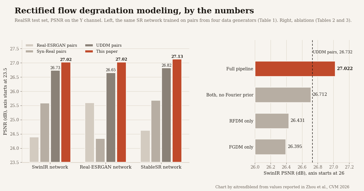
To test the synthetic data fairly, the authors followed UDDM and trained three very different SR networks on pairs from four generators. SwinIR from Liang and colleagues represents transformers, Real-ESRGAN represents GANs and StableSR from Wang and colleagues represents diffusion.
| SR network (pair source) | RealSR PSNR ↑ | SSIM ↑ | LPIPS ↓ | FID ↓ | DRealSR PSNR ↑ | SSIM ↑ | LPIPS ↓ | FID ↓ |
|---|---|---|---|---|---|---|---|---|
| SwinIR (Real-ESRGAN) | 24.395 | 0.7760 | 0.3037 | 119.43 | 26.944 | 0.8308 | 0.3219 | 139.18 |
| SwinIR (Syn-Real) | 25.589 | 0.7687 | 0.3835 | 163.13 | 28.301 | 0.8309 | 0.3801 | 154.59 |
| SwinIR (UDDM) | 26.732 | 0.7913 | 0.2652 | 105.92 | 29.247 | 0.8386 | 0.2709 | 118.09 |
| SwinIR (this paper) | 27.022 | 0.7981 | 0.2517 | 101.83 | 29.514 | 0.8409 | 0.2510 | 112.11 |
| Real-ESRGAN (Real-ESRGAN) | 25.600 | 0.7587 | 0.2749 | 138.94 | 28.549 | 0.8043 | 0.2820 | 146.94 |
| Real-ESRGAN (Syn-Real) | 24.341 | 0.7370 | 0.3021 | 159.44 | 27.483 | 0.7899 | 0.3306 | 171.89 |
| Real-ESRGAN (UDDM) | 26.651 | 0.7769 | 0.2061 | 102.43 | 29.176 | 0.8032 | 0.2645 | 150.44 |
| Real-ESRGAN (this paper) | 27.024 | 0.7932 | 0.1915 | 94.90 | 29.323 | 0.8051 | 0.2412 | 142.74 |
| StableSR (Real-ESRGAN) | 24.629 | 0.7035 | 0.3014 | 133.92 | 27.846 | 0.7412 | 0.3337 | 152.62 |
| StableSR (Syn-Real) | 25.679 | 0.7302 | 0.3680 | 165.62 | 28.621 | 0.7952 | 0.3892 | 183.45 |
| StableSR (UDDM) | 26.820 | 0.7768 | 0.2514 | 128.11 | 29.678 | 0.8267 | 0.2567 | 140.55 |
| StableSR (this paper) | 27.128 | 0.7798 | 0.2333 | 112.45 | 29.792 | 0.8313 | 0.2396 | 132.17 |
Table 1 of the paper. PSNR and SSIM are computed on the Y channel of YCbCr over a central crop, LPIPS and FID on RGB.
The pattern is consistent. For every network, on both datasets and all four metrics, the new pairs give the best result. The fidelity margins over UDDM are small, 0.29 dB and 0.0068 SSIM for SwinIR on RealSR and 0.267 dB and 0.0023 SSIM on DRealSR. The perceptual margins over older generators are large. With StableSR, the new pairs cut LPIPS by 0.1347 and FID by 53.17 on RealSR compared with Syn-Real pairs, and by 0.1496 and 51.28 on DRealSR.
Averages can hide a lot, so the authors also looked image by image. With StableSR, 88 percent of RealSR test images gain more than 0.1 dB over the UDDM trained model, and 90 percent of DRealSR images gain more than 0.05 dB. The improvement is broad rather than driven by a few outliers, which makes a small average gain more believable.
The visual comparisons tell a similar story. Networks trained on Real-ESRGAN pairs add artifacts to foliage, while those trained on Syn-Real and UDDM pairs blur it. Text and architectural lines hold their shape better with the new pairs. Looking at the synthetic low resolution images themselves, Real-ESRGAN pairs contain noise patterns that real photos do not, Syn-Real distorts structure and UDDM loses texture. A t-SNE plot of the generated images shows the new method overlapping most closely with real low resolution images.
A user study adds a human check. The authors collected 347 valid responses from 54 participants comparing StableSR outputs, and their method was preferred in 80 percent of cases overall.
Cost
| Degradation model | Parameters | FLOPs | Runtime (s) |
|---|---|---|---|
| Syn-Real | 120.7M | 2491G | 2.112 |
| UDDM | 135.4M | 2523G | 2.443 |
| FGDM | 953k | 114G | 0.612 |
| RFDM | 68.3M | 1562G | 1.441 |
| FGDM + RFDM | 69.4M | 1676G | 1.947 |
Table 4 of the paper. The paper does not state the image size behind the runtime figures.
The combined model is about half the size of UDDM and uses roughly a third fewer FLOPs, though its runtime advantage is smaller, 1.947 seconds against 2.443. Almost all the weight sits in the RFDM UNet. Since this cost is paid once, when generating training data, it matters less than inference cost would for the SR network itself.
What the ablations reveal
| Configuration (SwinIR) | RealSR PSNR/SSIM | DRealSR PSNR/SSIM |
|---|---|---|
| FGDM only | 26.395 / 0.7784 | 28.752 / 0.8263 |
| RFDM only | 26.431 / 0.7791 | 28.761 / 0.8277 |
| Both modules, no Fourier prior | 26.712 / 0.7891 | 29.211 / 0.8335 |
| Both modules with Fourier prior | 27.022 / 0.7981 | 29.514 / 0.8409 |
| UDDM pairs, for reference | 26.732 / 0.7913 | 29.247 / 0.8386 |
Tables 2 and 3 of the paper, with the UDDM row from Table 1 added for comparison.
This table is the most revealing part of the paper, and it rewards a close read. Each module alone improves on Real-ESRGAN and Syn-Real pairs, but neither reaches UDDM. FGDM alone scores 26.395 dB on RealSR and RFDM alone scores 26.431 dB, both below UDDM’s 26.732. Even with both modules, removing the Fourier phase guidance leaves the pipeline at 26.712 dB on RealSR and 29.211 dB on DRealSR, just under UDDM on both datasets.
So the lead over the previous best comes entirely from combining the pieces, with the phase prior as the deciding ingredient. That is not a flaw. The authors designed the modules to be complementary, and the numbers bear that out. It does mean that anyone hoping to borrow just the rectified flow, or just the DT-LR trick, should expect results closer to the prior state of the art than to this paper’s headline.
“After repeated up and down sampling operations, LR images with different degradations transform into similar degradations.”Zhou, Qin, Chen, He and Zhu, Computational Visual Media, 2026
Where we would push back
The phase used in training and synthesis differs. During training, FGDM takes its phase from the real low resolution target. During synthesis, it takes the phase from a clean bilinear downsample. The amplitude and phase swap experiment holds up well for blur, which mostly changes amplitude. Noise is another matter. Random sensor noise scrambles the phase at high frequencies, so the training phase contains a noise signature that the synthesis phase never has. In our small toy with signal dependent noise, combining bilinear amplitude with real phase produced an image much closer to the real noisy image, 36.48 dB, than to the bilinear one, 27.71 dB. That toy proves nothing about real cameras, but it suggests that some of the degradation travels in the phase, and that RFDM may be doing more of the noise modeling than the Fourier framing implies.
Evaluation stays inside the training domain. The degradation modules learn from the RealSR and DRealSR training sets and are then tested on the RealSR and DRealSR test sets, which come from the same capture setups. That is the standard protocol and it matches UDDM, but it measures how well the method learns a known camera from unpaired data, not how well a model trained this way handles an unseen camera. Photos from phones, webcams or old scanners are the real test, and the paper does not include one.
Perceptual quality depends on the network. Within each network the new pairs win, but across networks the picture is mixed. StableSR trained on the new pairs has the best PSNR on RealSR at 27.128 dB, yet its FID of 112.45 is worse than Real-ESRGAN trained on the same data at 94.90. Better data does not remove the tradeoffs between architectures.
Details for reproduction are thin. The paper does not report learning rates, the scale factor used inside each up and down sampling round, or the UNet configuration, and we could not find a code release. The user study, at 54 participants and one SR network, is useful but small.
Treat this as a clear, consistent improvement in synthetic training data for cameras whose real low resolution photos you already have. The gain over the best prior generator is about a quarter to a third of a decibel, larger on perceptual metrics against older generators, and it relies on all three components working together.
Limitations the authors acknowledge
Too few real low resolution images. The high resolution pool is large, 800 images from DIV2K, 2560 from Flickr2K and 10,324 from OutdoorSceneTraining. The real low resolution pool is tiny by comparison, 495 images from RealSR and 840 from DRealSR. That imbalance limits the variety of degradations and scenes the model can learn from, and the authors name it as the main direction for future work. It is also a reminder of why the method matters. Real low resolution data is scarce everywhere in super resolution research.
DT-LR was found by trial and error. The choice of bilinear resampling and ten rounds came from extensive manual search across sampling methods, scale factors and counts, which was slow and expensive. The authors say plainly that the current strategy may not be theoretically optimal, only that it beats the approaches used in UDDM and Syn-Real, and they hope to find a more principled way to build these intermediate images.
Where this fits and who should care
For practitioners the appeal is modularity. Nothing about the SR network changes. If you already train SwinIR, Real-ESRGAN, StableSR or a compact model like the IQ-LUT lookup table network, you can swap in better training pairs and keep the rest of your pipeline. If you have a few hundred real photos from a target camera, a security system or a scanner, you can in principle learn its degradation without ever capturing aligned pairs.
The broader idea is the conversion from unpaired to paired learning. Destroying the information that differs between two domains, then restoring structure from a shared signal, gives aligned training data where none existed. Similar logic could help in endoscopy image restoration, where clean references are rare, or in the unsupervised hyperspectral setting behind EDIP-Net and BKSR. It also shows rectified flow as a practical tool for learning degradation, not only for generating images. Our generative and diffusion models archive collects related work in one place.
Reference implementation in PyTorch
The code below implements the full pipeline in one file. It contains DT-LR generation, Fourier amplitude and phase helpers, a MambaIR style residual state space block with a four direction selective scan, AENet and FGDM, a time conditioned UNet velocity field, RFDM with its training loss and Euler sampler, the two stage degradation training loop with the paper’s augmentations, pair synthesis, a small stand in SR network, Y channel PSNR and SSIM on a central crop, and a smoke test on dummy data.
The smoke test builds a hidden camera from blur, decimation, a slight color cast and signal dependent noise, and uses it only to make unpaired real low resolution images and a held out test set. The selective scan is written as a plain Python loop, which is exact but slow, so for full size training replace it with the CUDA kernel from the mamba_ssm package. Values the paper does not report, including learning rates and the scale factor inside each DT-LR round, are marked in the code as our choices.
"""
Unsupervised real-world image super-resolution via rectified flow degradation modeling.
Reference PyTorch implementation of the pipeline in
    Zhou, Qin, Chen, He, Zhu. Computational Visual Media 12(4), 1035-1051, 2026.
    https://doi.org/10.26599/CVM.2026.9450559

Pipeline (Algorithm 1 of the paper)
    1. DT-LR      repeated bilinear up and down sampling (N = 10) pushes differently degraded
                  LR images toward a common, "degradation transformed" state
    2. FGDM       Fourier prior guided degradation module. AENet (conv + residual state space
                  blocks) processes DT-LR, its FFT amplitude is kept, the FFT phase is taken
                  from a structure reference, and the IFFT gives a preliminary degraded LR.
                  Trained with L1 against the real LR image.
    3. RFDM       rectified flow degradation module. A time conditioned UNet learns the
                  velocity from X0 = FGDM output + lambda * noise to X1 = real LR (Eq. 5-7).
                  Synthesis integrates the ODE with K = 20 Euler steps (Eq. 8).
    4. SR model   any off-the-shelf SR network is trained on (synthetic LR, HR) pairs.

Honest notes
    * The residual state space block (RSSB) follows MambaIR. Its selective scan is written
      in plain PyTorch with a sequential loop, which is exact but slow. For full size training
      swap `selective_scan` for the CUDA kernel in the `mamba_ssm` package.
    * Items the paper does not specify, and which we therefore chose: the up/down scale
      factor inside DT-LR (2), the AENet global residual, the UNet widths, learning rates,
      and the SR network used in the smoke test (a tiny residual CNN standing in for SwinIR,
      Real-ESRGAN or StableSR).
    * LPIPS and FID need pretrained networks; `evaluate` reports PSNR and SSIM on the
      Y channel of YCbCr over a central crop, as the paper does for fidelity metrics.
"""
import math
import torch
import torch.nn as nn
import torch.nn.functional as F

# ---------------------------------------------------------------------------
# 1. Degradation transformed LR (DT-LR)
# ---------------------------------------------------------------------------

def dt_lr(x: torch.Tensor, n: int = 10, factor: int = 2, mode: str = "bilinear") -> torch.Tensor:
    """Apply n rounds of (upsample by `factor`, then downsample back). Output keeps x's size."""
    h, w = x.shape[-2:]
    for _ in range(n):
        x = F.interpolate(x, scale_factor=factor, mode=mode, align_corners=False)
        x = F.interpolate(x, size=(h, w), mode=mode, align_corners=False)
    return x


def bilinear_down(y: torch.Tensor, scale: int = 4) -> torch.Tensor:
    return F.interpolate(y, scale_factor=1 / scale, mode="bilinear", align_corners=False, antialias=True)

# ---------------------------------------------------------------------------
# 2. Fourier helpers
# ---------------------------------------------------------------------------

def amp_phase(x: torch.Tensor, eps: float = 1e-8):
    X = torch.fft.fft2(x, norm="ortho")
    amp = torch.sqrt(X.real ** 2 + X.imag ** 2 + eps)
    pha = torch.atan2(X.imag, X.real + 0.0)
    return amp, pha


def combine(amp: torch.Tensor, pha: torch.Tensor) -> torch.Tensor:
    return torch.fft.ifft2(torch.polar(amp, pha), norm="ortho").real

# ---------------------------------------------------------------------------
# 3. Residual state space block (MambaIR style) for AENet
# ---------------------------------------------------------------------------

def selective_scan(u, delta, A, B, C, D):
    """Mamba S6 recurrence, h_t = exp(delta_t A) h_{t-1} + delta_t B_t u_t,  y_t = C_t h_t + D u_t.
    u, delta (b, d, L)   A (d, n)   B, C (b, n, L)   D (d,)"""
    b, d, L = u.shape
    dA = torch.exp(delta.unsqueeze(-1) * A[None, :, None, :])      # (b, d, L, n)
    dBu = delta.unsqueeze(-1) * B.transpose(1, 2).unsqueeze(1) * u.unsqueeze(-1)
    h = u.new_zeros(b, d, A.shape[1])
    ys = []
    for t in range(L):
        h = dA[:, :, t] * h + dBu[:, :, t]
        ys.append((h * C[:, :, t].unsqueeze(1)).sum(-1))
    return torch.stack(ys, -1) + u * D[None, :, None]


class SS2D(nn.Module):
    """2D selective scan over four directions (row major, column major, and their reverses)."""

    def __init__(self, dim, d_state=16, expand=2):
        super().__init__()
        di = dim * expand
        self.di, self.n = di, d_state
        self.dt_rank = math.ceil(dim / 16)
        self.in_proj = nn.Linear(dim, 2 * di)
        self.dwconv = nn.Conv2d(di, di, 3, padding=1, groups=di)
        self.x_proj = nn.Parameter(torch.randn(4, self.dt_rank + 2 * d_state, di) * di ** -0.5)
        self.dt_proj_w = nn.Parameter(torch.randn(4, di, self.dt_rank) * self.dt_rank ** -0.5)
        dt = torch.exp(torch.rand(4, di) * (math.log(0.1) - math.log(0.001)) + math.log(0.001))
        self.dt_proj_b = nn.Parameter(dt + torch.log(-torch.expm1(-dt)))    # inverse softplus
        self.A_log = nn.Parameter(torch.log(torch.arange(1, d_state + 1).float()).repeat(4 * di, 1))
        self.D = nn.Parameter(torch.ones(4 * di))
        self.out_norm = nn.LayerNorm(di)
        self.out_proj = nn.Linear(di, dim)

    def forward(self, x):                                                   # x (b, h, w, c)
        b, h, w, _ = x.shape
        xz = self.in_proj(x)
        xi, z = xz.chunk(2, -1)
        xi = F.silu(self.dwconv(xi.permute(0, 3, 1, 2)))                    # (b, di, h, w)
        L = h * w
        row = xi.flatten(2)
        col = xi.transpose(2, 3).flatten(2)
        seqs = torch.stack([row, col, row.flip(-1), col.flip(-1)], 1)       # (b, 4, di, L)
        A = -torch.exp(self.A_log).view(4, self.di, self.n)
        outs = []
        for k in range(4):
            u = seqs[:, k]
            proj = torch.einsum("bdl,cd->bcl", u, self.x_proj[k])
            dt_r, Bm, Cm = torch.split(proj, [self.dt_rank, self.n, self.n], 1)
            delta = F.softplus(torch.einsum("brl,dr->bdl", dt_r, self.dt_proj_w[k]) + self.dt_proj_b[k][None, :, None])
            outs.append(selective_scan(u, delta, A[k], Bm, Cm, self.D.view(4, self.di)[k]))
        y = outs[0] + outs[2].flip(-1)
        yc = outs[1] + outs[3].flip(-1)
        y = y + yc.view(b, self.di, w, h).transpose(2, 3).flatten(2)
        y = self.out_norm(y.transpose(1, 2).view(b, h, w, self.di))
        return self.out_proj(y * F.silu(z))


class ChannelAttention(nn.Module):
    def __init__(self, c, r=16):
        super().__init__()
        self.net = nn.Sequential(nn.AdaptiveAvgPool2d(1), nn.Conv2d(c, max(c // r, 4), 1), nn.ReLU(inplace=True),
                                 nn.Conv2d(max(c // r, 4), c, 1), nn.Sigmoid())

    def forward(self, x):
        return x * self.net(x)


class RSSB(nn.Module):
    """Two residual branches with learnable scales (MambaIR).
    Branch 1, LayerNorm then SS2D for long range context.
    Branch 2, LayerNorm then conv then channel attention for local detail."""

    def __init__(self, dim):
        super().__init__()
        self.ln1, self.ln2 = nn.LayerNorm(dim), nn.LayerNorm(dim)
        self.ss2d = SS2D(dim)
        self.conv = nn.Sequential(nn.Conv2d(dim, dim // 3, 3, padding=1), nn.GELU(), nn.Conv2d(dim // 3, dim, 3, padding=1))
        self.ca = ChannelAttention(dim)
        self.s1 = nn.Parameter(torch.ones(dim))
        self.s2 = nn.Parameter(torch.ones(dim))

    def forward(self, x):                                                   # (b, c, h, w)
        t = x.permute(0, 2, 3, 1)
        t = t * self.s1 + self.ss2d(self.ln1(t))
        c = self.ln2(t).permute(0, 3, 1, 2)
        c = self.ca(self.conv(c)).permute(0, 2, 3, 1)
        t = t * self.s2 + c
        return t.permute(0, 3, 1, 2)


class AENet(nn.Module):
    """Amplitude enhancement network. Conv, n RSSBs, conv. Paper default n = 6, width 96."""

    def __init__(self, width=96, n_blocks=6, ch=3):
        super().__init__()
        self.head = nn.Conv2d(ch, width, 3, padding=1)
        self.body = nn.Sequential(*[RSSB(width) for _ in range(n_blocks)])
        self.tail = nn.Conv2d(width, ch, 3, padding=1)

    def forward(self, x):
        f = self.head(x)
        return x + self.tail(self.body(f) + f)                            # global residual (our choice)


class FGDM(nn.Module):
    """Fourier prior guided degradation module.
    amplitude  <- FFT(AENet(DT-LR))       learns what the degradation does to the spectrum
    phase      <- FFT(structure reference) real LR during training, bilinear LR of HR at synthesis
    output      = IFFT(amplitude, phase)"""

    def __init__(self, width=96, n_blocks=6):
        super().__init__()
        self.aenet = AENet(width, n_blocks)

    def forward(self, x_dt, phase_ref):
        amp, _ = amp_phase(self.aenet(x_dt))
        _, pha = amp_phase(phase_ref)
        return combine(amp, pha)

# ---------------------------------------------------------------------------
# 4. RFDM: rectified flow with a time conditioned UNet velocity field
# ---------------------------------------------------------------------------

def time_embedding(t, dim):
    half = dim // 2
    freqs = torch.exp(-math.log(10000) * torch.arange(half, device=t.device) / half)
    a = t[:, None] * 1000 * freqs[None]
    return torch.cat([a.sin(), a.cos()], -1)


class ResBlock(nn.Module):
    def __init__(self, cin, cout, tdim):
        super().__init__()
        self.n1, self.n2 = nn.GroupNorm(8, cin), nn.GroupNorm(8, cout)
        self.c1, self.c2 = nn.Conv2d(cin, cout, 3, padding=1), nn.Conv2d(cout, cout, 3, padding=1)
        self.t = nn.Linear(tdim, cout)
        self.skip = nn.Conv2d(cin, cout, 1) if cin != cout else nn.Identity()

    def forward(self, x, temb):
        h = self.c1(F.silu(self.n1(x))) + self.t(temb)[:, :, None, None]
        h = self.c2(F.silu(self.n2(h)))
        return h + self.skip(x)


class VelocityUNet(nn.Module):
    def __init__(self, ch=3, base=64, mults=(1, 2, 4)):
        super().__init__()
        self.tdim = base * 4
        self.tmlp = nn.Sequential(nn.Linear(base, self.tdim), nn.SiLU(), nn.Linear(self.tdim, self.tdim))
        self.base = base
        self.inp = nn.Conv2d(ch, base, 3, padding=1)
        chs = [base * m for m in mults]
        self.down, self.pools = nn.ModuleList(), nn.ModuleList()
        c = base
        for i, co in enumerate(chs):
            self.down.append(ResBlock(c, co, self.tdim))
            self.pools.append(nn.Conv2d(co, co, 3, stride=2, padding=1) if i < len(chs) - 1 else nn.Identity())
            c = co
        self.mid = ResBlock(c, c, self.tdim)
        self.up, self.ups = nn.ModuleList(), nn.ModuleList()
        for i, co in reversed(list(enumerate(chs))):
            self.up.append(ResBlock(c + co, co, self.tdim))
            self.ups.append(nn.Upsample(scale_factor=2, mode="nearest") if i > 0 else nn.Identity())
            c = co
        self.out = nn.Sequential(nn.GroupNorm(8, c), nn.SiLU(), nn.Conv2d(c, ch, 3, padding=1))

    def forward(self, x, t):
        temb = self.tmlp(time_embedding(t, self.base))
        h = self.inp(x)
        skips = []
        for blk, pool in zip(self.down, self.pools):
            h = blk(h, temb)
            skips.append(h)
            h = pool(h)
        h = self.mid(h, temb)
        for blk, up in zip(self.up, self.ups):
            h = blk(torch.cat([h, skips.pop()], 1), temb)
            h = up(h)
        return self.out(h)


class RFDM(nn.Module):
    def __init__(self, base=64, lam=0.1, steps=20):
        super().__init__()
        self.v = VelocityUNet(base=base)
        self.lam, self.steps = lam, steps

    def loss(self, x_bar, x_real):
        """Eq. 5-7. X0 = FGDM output + lambda * n,  X1 = real LR,  L2 on the constant velocity X1 - X0."""
        x0 = x_bar + self.lam * torch.randn_like(x_bar)
        t = torch.rand(x0.shape[0], device=x0.device)
        xt = t[:, None, None, None] * x_real + (1 - t[:, None, None, None]) * x0
        return F.mse_loss(self.v(xt, t), x_real - x0)

    @torch.no_grad()
    def sample(self, x_bar, steps=None):
        """Eq. 8. Euler integration from X0 = x_bar + lambda * n to X1 in K steps."""
        K = steps or self.steps
        x = x_bar + self.lam * torch.randn_like(x_bar)
        for i in range(K):
            t = torch.full((x.shape[0],), i / K, device=x.device)
            x = x + self.v(x, t) / K
        return x

# ---------------------------------------------------------------------------
# 5. The full degradation pipeline
# ---------------------------------------------------------------------------

class RFDegradation(nn.Module):
    def __init__(self, width=96, n_blocks=6, unet_base=64, lam=0.1, steps=20, n_updown=10, scale=4):
        super().__init__()
        self.fgdm = FGDM(width, n_blocks)
        self.rfdm = RFDM(unet_base, lam, steps)
        self.n_updown, self.scale = n_updown, scale

    def fgdm_loss(self, x_real):
        """Stage 1. L1 between FGDM(DT-LR(real), phase(real)) and the real LR."""
        x_bar = self.fgdm(dt_lr(x_real, self.n_updown), x_real)
        return F.l1_loss(x_bar, x_real)

    def rfdm_loss(self, x_real):
        """Stage 2. FGDM is frozen, RFDM learns the flow from its output to the real LR."""
        with torch.no_grad():
            x_bar = self.fgdm(dt_lr(x_real, self.n_updown), x_real)
        return self.rfdm.loss(x_bar, x_real)

    @torch.no_grad()
    def synthesize(self, y_hr):
        """HR -> bilinear LR -> DT-LR -> FGDM (phase of the bilinear LR) -> RFDM ODE -> synthetic LR."""
        lr_bi = bilinear_down(y_hr, self.scale)
        x_bar = self.fgdm(dt_lr(lr_bi, self.n_updown), lr_bi)
        return self.rfdm.sample(x_bar).clamp(0, 1)

# ---------------------------------------------------------------------------
# 6. A stand in SR network, training loops and evaluation
# ---------------------------------------------------------------------------

class TinySR(nn.Module):
    """Small residual CNN with pixel shuffle. Replace with SwinIR, Real-ESRGAN or StableSR."""

    def __init__(self, scale=4, c=48, n=6):
        super().__init__()
        self.head = nn.Conv2d(3, c, 3, padding=1)
        self.body = nn.Sequential(*[nn.Sequential(nn.Conv2d(c, c, 3, padding=1), nn.ReLU(True), nn.Conv2d(c, c, 3, padding=1)) for _ in range(n)])
        self.up = nn.Sequential(nn.Conv2d(c, 3 * scale * scale, 3, padding=1), nn.PixelShuffle(scale))
        self.scale = scale

    def forward(self, x):
        f = self.head(x)
        for blk in self.body:
            f = f + blk(f)
        return self.up(f) + F.interpolate(x, scale_factor=self.scale, mode="bilinear", align_corners=False)


def augment(x):
    """Random rotation by 0, 90, 180 or 270 degrees and random horizontal flip (Sec. 4.1)."""
    k = torch.randint(4, (1,)).item()
    x = torch.rot90(x, k, (-2, -1))
    return x.flip(-1) if torch.rand(1).item() < 0.5 else x


def train_degradation(model, real_lr, epochs_fgdm=1000, epochs_rfdm=1000, bs=8, lr=2e-4, log=100):
    """Paper setting, 1000 epochs each with Adam(beta1 0.9, beta2 0.999). Learning rate not reported."""
    opt = torch.optim.Adam(model.fgdm.parameters(), lr=lr, betas=(0.9, 0.999))
    for ep in range(1, epochs_fgdm + 1):
        for i in range(0, len(real_lr), bs):
            loss = model.fgdm_loss(augment(real_lr[i:i + bs]))
            opt.zero_grad(); loss.backward(); opt.step()
        if log and ep % log == 0:
            print(f"FGDM epoch {ep}  L1 {loss.item():.4f}")
    model.fgdm.requires_grad_(False)
    opt = torch.optim.Adam(model.rfdm.parameters(), lr=lr, betas=(0.9, 0.999))
    for ep in range(1, epochs_rfdm + 1):
        for i in range(0, len(real_lr), bs):
            loss = model.rfdm_loss(augment(real_lr[i:i + bs]))
            opt.zero_grad(); loss.backward(); opt.step()
        if log and ep % log == 0:
            print(f"RFDM epoch {ep}  L2 {loss.item():.4f}")
    return model


def train_sr(sr, lr_imgs, hr_imgs, epochs=100, bs=8, lr=2e-4):
    opt = torch.optim.Adam(sr.parameters(), lr=lr)
    for _ in range(epochs):
        perm = torch.randperm(len(lr_imgs))
        for i in range(0, len(lr_imgs), bs):
            idx = perm[i:i + bs]
            loss = F.l1_loss(sr(lr_imgs[idx]), hr_imgs[idx])
            opt.zero_grad(); loss.backward(); opt.step()
    return sr


def rgb_to_y(x):
    return (16 + 65.481 * x[:, 0] + 128.553 * x[:, 1] + 24.966 * x[:, 2]) / 255.0


def center_crop(x, frac=0.5):
    h, w = x.shape[-2:]
    ch, cw = int(h * frac), int(w * frac)
    return x[..., (h - ch) // 2:(h - ch) // 2 + ch, (w - cw) // 2:(w - cw) // 2 + cw]


def psnr_y(a, b):
    return (10 * torch.log10(1.0 / F.mse_loss(rgb_to_y(a), rgb_to_y(b), reduction="none").mean((-2, -1)))).mean()


def ssim_y(a, b, win=11):
    a, b = rgb_to_y(a)[:, None], rgb_to_y(b)[:, None]
    g = torch.exp(-((torch.arange(win) - win // 2) ** 2) / (2 * 1.5 ** 2)); g = g / g.sum()
    k = (g[:, None] * g[None])[None, None]
    f = lambda t: F.conv2d(t, k, padding=win // 2)
    ma, mb = f(a), f(b)
    va, vb, cab = f(a * a) - ma ** 2, f(b * b) - mb ** 2, f(a * b) - ma * mb
    C1, C2 = 0.01 ** 2, 0.03 ** 2
    return (((2 * ma * mb + C1) * (2 * cab + C2)) / ((ma ** 2 + mb ** 2 + C1) * (va + vb + C2))).mean()


@torch.no_grad()
def evaluate(sr, lr_test, hr_test):
    out = sr(lr_test).clamp(0, 1)
    out, hr = center_crop(out), center_crop(hr_test)
    return psnr_y(out, hr).item(), ssim_y(out, hr).item()

# ---------------------------------------------------------------------------
# 7. Smoke test on dummy data
# ---------------------------------------------------------------------------

def smooth_textures(n, size, seed):
    g = torch.Generator().manual_seed(seed)
    x = torch.rand(n, 3, size // 8, size // 8, generator=g)
    x = F.interpolate(x, size=size, mode="bicubic", align_corners=False)
    stripes = torch.sin(torch.linspace(0, 12 * math.pi, size))[None, None, None] * torch.rand(n, 3, 1, 1, generator=g)
    return (0.7 * x + 0.3 * (stripes + 1) / 2).clamp(0, 1)


def hidden_camera(y, seed=0):
    """The 'unknown' real world degradation, used only to create real LR and test pairs.
    Gaussian blur, 4x decimation, a slight color cast and signal dependent noise."""
    g = torch.Generator().manual_seed(seed)
    k = torch.exp(-(torch.arange(7) - 3.0) ** 2 / (2 * 1.6 ** 2)); k = (k[:, None] * k[None]) / k.sum() ** 2
    yb = F.conv2d(F.pad(y, (3, 3, 3, 3), mode="reflect"), k.expand(3, 1, 7, 7), groups=3)
    x = yb[..., ::4, ::4] * torch.tensor([1.03, 1.0, 0.95])[None, :, None, None]
    return (x + 0.03 * torch.sqrt(x.clamp(min=1e-4)) * torch.randn(x.shape, generator=g)).clamp(0, 1)


def hf_energy(x):
    return (x[..., 1:, :] - x[..., :-1, :]).abs().mean().item() + (x[..., 1:] - x[..., :-1]).abs().mean().item()


if __name__ == "__main__":
    torch.manual_seed(0)
    S = 64                                                                   # HR size, LR is S/4

    # Unpaired training data: real LR images come from different scenes than the HR set
    hr_train = smooth_textures(24, S, seed=1)
    real_lr = hidden_camera(smooth_textures(24, S, seed=2), seed=3)
    hr_test = smooth_textures(8, S, seed=4)
    lr_test = hidden_camera(hr_test, seed=5)

    # (a) DT-LR convergence, the observation behind Fig. 3
    y = smooth_textures(8, S, seed=6)
    lr_real, lr_bi = hidden_camera(y, seed=7), bilinear_down(y)
    for n in (0, 1, 5, 10):
        p = psnr_y(dt_lr(lr_real, n), dt_lr(lr_bi, n)).item()
        print(f"DT-LR rounds {n:2d}  PSNR(real, bilinear) {p:6.2f} dB  high frequency energy {hf_energy(dt_lr(lr_real, n)):.4f}")

    # (b) Fourier amplitude and phase swap, the observation behind Fig. 5
    a_amp, a_pha = amp_phase(lr_real)
    b_amp, b_pha = amp_phase(lr_bi)
    swapped = combine(b_amp, a_pha)
    print(f"amplitude of bilinear + phase of real, PSNR to bilinear {psnr_y(swapped, lr_bi).item():.2f} dB, to real {psnr_y(swapped, lr_real).item():.2f} dB")

    # (c) Train the degradation modules (tiny sizes and few epochs for the smoke test)
    model = RFDegradation(width=24, n_blocks=2, unet_base=32, lam=0.1, steps=20)
    print("parameters FGDM", sum(p.numel() for p in model.fgdm.parameters()),
          " RFDM", sum(p.numel() for p in model.rfdm.parameters()))
    train_degradation(model, real_lr, epochs_fgdm=20, epochs_rfdm=40, bs=8, lr=1e-3, log=10)

    # (d) Synthesize LR for the HR set and compare statistics with real LR
    syn_lr = model.synthesize(hr_train)
    bic_lr = bilinear_down(hr_train)
    print(f"high frequency energy  real LR {hf_energy(real_lr):.4f}  synthetic LR {hf_energy(syn_lr):.4f}  bilinear LR {hf_energy(bic_lr):.4f}")
    print(f"mean color  real {real_lr.mean((0, 2, 3)).tolist()}")
    print(f"mean color  synthetic {syn_lr.mean((0, 2, 3)).tolist()}")

    # (e) Train the same SR network on synthetic pairs and on bilinear pairs, test on hidden camera LR
    torch.manual_seed(0)
    sr_syn = train_sr(TinySR(), syn_lr, hr_train, epochs=60)
    torch.manual_seed(0)
    sr_bic = train_sr(TinySR(), bic_lr, hr_train, epochs=60)
    print("SR trained on synthetic pairs, test PSNR/SSIM (Y, center crop):", [round(v, 4) for v in evaluate(sr_syn, lr_test, hr_test)])
    print("SR trained on bilinear pairs,  test PSNR/SSIM (Y, center crop):", [round(v, 4) for v in evaluate(sr_bic, lr_test, hr_test)])
    print("shapes", tuple(real_lr.shape), tuple(syn_lr.shape), tuple(hr_train.shape))
Running the file takes about three minutes on a laptop CPU and prints the following. The first block reproduces the paper’s DT-LR convergence trend in miniature and shows the drop in high frequency energy that comes with it. The second block is the amplitude and phase swap discussed above. The toy training runs are far too short and small to say anything about the benchmark numbers. They only confirm that every loss trains and every stage connects.
Conclusion
Zhou, Qin, Chen, He and Zhu tackle a problem that has shadowed super resolution for a decade. Networks learn from pairs, and the pairs they learn from rarely look like the photos they will meet. Their answer is to learn the degradation of real cameras from unpaired data and to manufacture training pairs that carry it, leaving the SR network itself untouched. Across three very different networks and two real world benchmarks, the synthetic pairs consistently give the best results.
The conceptual move is to create correspondence where none exists. Repeated bilinear resampling pushes every image toward a shared DT-LR state, and Fourier phase restores the structure that resampling erases. That produces, for each real photo, an aligned input from which its degradation can be learned by plain regression. Rectified flow then provides a stable, fast way to add the realism a deterministic module cannot, with straight paths that need only 20 integration steps.
The ideas should travel. Any restoration task that has plenty of clean images and a modest number of degraded ones, from medical scans to satellite images to archival film, faces the same unpaired problem. A shared intermediate domain plus a structure prior is a pattern worth trying well beyond super resolution, and rectified flow is a natural fit whenever the source and target are already close.
The limits deserve equal weight. Gains over the best prior generator are a few tenths of a decibel. The evaluation stays within the cameras used for training, so generalization to new devices remains open. Each component alone falls short of the prior state of the art, the phase guidance may carry more degradation than the framing suggests, and without code or learning rates, independent reproduction will take work. The scarcity of real low resolution data, which the authors highlight themselves, caps how much variety any such model can learn.
The next steps are clear. Test on devices that were never seen in training, grow the pool of real low resolution images, and replace the hand tuned DT-LR recipe with something learned or derived. What this paper shows is that the most effective way to improve a super resolution network may be to leave the network alone and teach the data to look like the real world.
Frequently asked questions
What is rectified flow degradation modeling for super resolution?
It is a method that learns how real cameras degrade images and applies that learned degradation to clean high resolution photos to create realistic low resolution training pairs. A rectified flow, a generative model that moves samples along straight paths, refines an initial degradation estimate into one that matches real camera output.
Why does unsupervised real world super resolution matter?
Networks trained on clean, mathematically downsampled images often fail on real photos, which carry mixed blur, sensor noise and compression. Capturing aligned real pairs requires special hardware. Unsupervised methods learn from unpaired photos, so they can adapt to a camera using only its own low resolution images.
What is a DT-LR image?
DT-LR stands for degradation transformed low resolution image. It is made by upsampling and downsampling an image with bilinear interpolation ten times. Images with different degradations become similar after this process, so DT-LR serves as a shared starting point for real photos and for images derived from clean high resolution sources.
Why does the method use Fourier phase?
Swapping Fourier amplitude between two differently degraded images mostly swaps their degradation, while phase mostly carries structure. The Fourier module therefore learns the degradation in the amplitude and takes the phase from a structure reference, which restores detail that repeated resampling removes.
How much does the method improve super resolution results?
With SwinIR it improves PSNR over UDDM generated pairs by 0.29 dB on RealSR and 0.267 dB on DRealSR, and it leads on PSNR, SSIM, LPIPS and FID for SwinIR, Real-ESRGAN and StableSR on both datasets. Gains are larger on perceptual metrics against older generators such as Syn-Real.
Can I use this with my own super resolution network?
Yes. The method only generates training pairs, so any supervised super resolution network can be trained on them without architectural changes. You need a set of real low resolution images from the target camera and a separate set of clean high resolution images.
Read the full paper
The article is open access under a Creative Commons Attribution license in Computational Visual Media, with the full method, ablations and visual comparisons on RealSR and DRealSR.
Zhou, H., Qin, J., Chen, L., He, J., and Zhu, X. Unsupervised real world image super resolution via rectified flow degradation modeling. Computational Visual Media, Vol. 12, No. 4, August 2026, pages 1035 to 1051. DOI 10.26599/CVM.2026.9450559.
This analysis is based on the published paper and an independent evaluation of its claims.