
- In context learning
- LLM graph reasoning
- Demonstration selection
- Benchmarks
- Linear attention
- Evaluation
- PyTorch
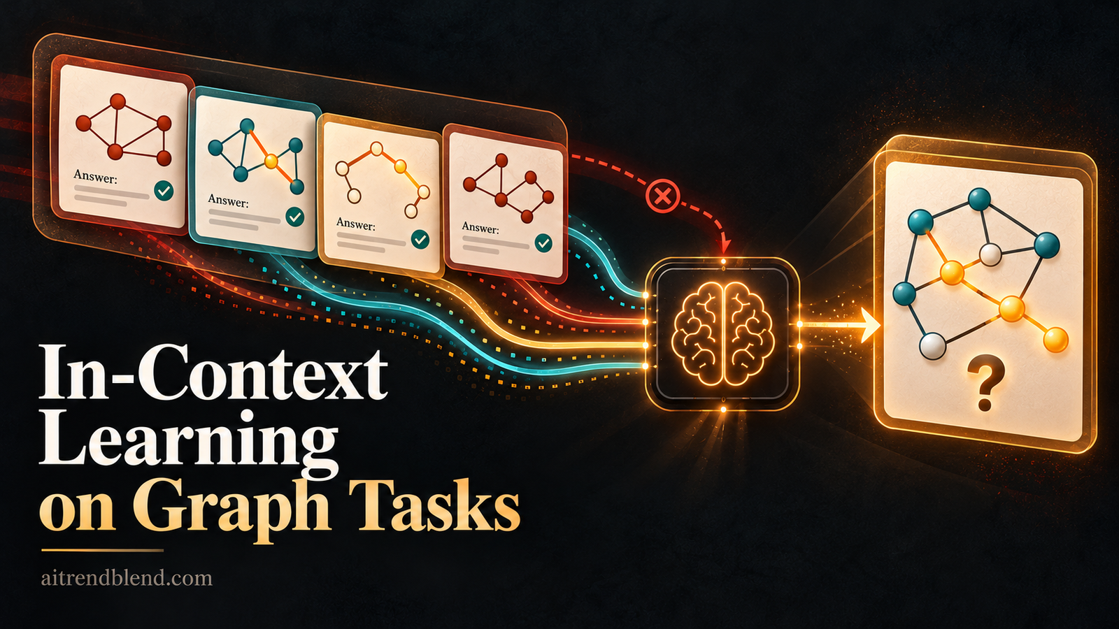
A developer wants a language model to answer questions about a network. Is node 14 connected to node 3. What is the shortest route between two depots. Does this dependency graph have a valid build order. The edges go into the prompt as plain text, and following standard advice, the developer adds four solved examples first. On some questions accuracy jumps. On others, especially the hardest ones, it drops, and nobody can say in advance which will happen.
A team led by Chunhui Zhang and Lizhong Ding at the Beijing Institute of Technology, with colleagues at Jinan University and Guilin University of Electronic Technology, set out to turn that guesswork into something systematic. They propose a formulation of in context learning on graph tasks, a theorem about how demonstrations change predictions, and two new benchmarks that vary one factor at a time. The benchmarks are the most useful part. The theory, and parts of the evaluation, need more care than the paper gives them.
Key points
- The study indexes every demonstration by three factors, how many there are, which graph they use and which task they solve, and builds two benchmarks with 17,155 graph questions to vary each factor separately.
- Across five models, more demonstrations usually help weaker models, but every model loses accuracy on Hamiltonian path questions as demonstrations are added. LLaMa3 8B falls from 69.19 to 33.33 percent.
- The strongest models, GPT-4o and Qwen3 32B, score highest with no demonstrations on average. Our recomputation finds GPT-4o’s eight demonstration average is 95.76, not the printed 96.76.
- Theorem 1, which says a demonstration acts like a rank one weight update, holds for any vectors whatsoever. The substantive claim sits in an assumption, which we show is exact for linear attention and only rough for softmax attention.
- Read literally, the paper’s own update rule predicts that models copy the majority answer of their demonstrations, a plausible explanation for the Hamiltonian collapse that the paper does not test.
- In the public code at commit 026556a, answers are graded by the evaluated model itself acting as a judge at temperature 1, while the paper describes rule based grading.
Why graph questions are hard for language models
Large language models read text one token at a time. A graph written as text, a list such as 0 to 3, 3 to 7, 7 to 2, loses the property that makes graphs useful, that any node can be reached from any other through structure the reader has to reconstruct. NLGraph, from Wang and colleagues, and GPT4Graph, from Guo and colleagues, both showed that models handle simple questions such as cycle detection reasonably well and struggle badly with harder ones such as Hamiltonian paths. Fatemi, Halcrow and Perozzi found that even the way edges are serialised changes the answers.
In context learning, the trick of adding solved examples to the prompt, should help. It does help on many language tasks, as Brown and colleagues showed with GPT-3. But on graphs the evidence is mixed. NLGraph found demonstrations did not help on complex graph tasks, and GPT4Graph reported cases where they introduced noise. Methods such as RGER and GraphIC try to choose better demonstrations, and PRODIGY builds graphs over demonstrations themselves. What has been missing is a controlled answer to a simpler question. When you hold everything else fixed, what does each property of a demonstration do?
The formulation and the theorem
Three indices for every demonstration
The paper writes each demonstration as \(Q^k_i(G_j)\) with answer \(A_{ijk}\), where \(j\) picks the graph, \(k\) picks the task category such as shortest path, and \(i\) counts demonstrations within that graph and task pair. The full context is the union over all graphs and tasks.
Writing it this way is simple, but it is genuinely helpful. It makes clear that a prompt can mix demonstrations from the query’s own graph and from other graphs, and from the query’s task and from other tasks, and that each of those choices is a separate experimental variable.
Demonstrations as a weight update
The model is abstracted as a function of a query embedding \(\phi(Q(G))\) passed through a weight matrix \(W\) and the rest of the network \(\theta\). Demonstrations change the embedding the network sees, from \(\phi(Q(G))\) to \(\phi(C, Q(G))\). Theorem 1 then says the same output can be produced without the demonstrations by updating the weights.
Theorem 2 extends this to many demonstrations by induction. Then Lemma 1 adds the step that gives the theory its content. It assumes the demonstration induced shift takes a specific form.
In words, each demonstration pushes the prediction in the direction of its answer, \(\phi(A)\), scaled by how similar its question is to the query, \(\phi(Q_i)^{\top}\phi(Q)\). From this the paper derives three assertions. The number of demonstrations matters, structural similarity between demonstration graphs and the query graph matters, and the task categories of demonstrations interact with the query’s task.
What Theorem 1 does and does not say
This is not a small distinction. Multiply \(\Delta W\) by \(\phi(Q)\) and the fraction cancels, leaving \(\Delta W\phi(Q) = W\Delta\phi\). That is true for any matrix \(W\) and any two vectors \(\phi(Q)\) and \(\phi(C, Q)\). Nothing about transformers, attention or graphs is used. We checked it with random numbers, a random 32 by 64 matrix and two random 64 dimensional vectors, and the identity held to an error of 2.9 times 10 to the minus 6, with \(\Delta W\) of rank one, exactly as stated.
The same observation appears in recent work on implicit weight updates in transformers, and it is a useful reframing. But it is a change of bookkeeping, not a discovery about the model. The real claim is Lemma 1, which the paper itself labels an assumption and notes does not require that models actually compute it. So we tested when it holds.
For a single attention layer without softmax, where the weight on each demonstration is the raw query key product, the shift that attention adds to the query position has exactly the Lemma 1 form. Our check found a cosine similarity of 1.000 between the two across 20 random layers. With the softmax that real language models use, the average cosine dropped to 0.56. The softmax renormalises the weights across demonstrations, so adding a demonstration also reduces the influence of all the others. Lemma 1 is therefore a linear attention picture of in context learning. It is a reasonable first approximation, not a derivation about the LLMs that were tested.
The theorem holds for any vectors. The insight, if there is one, lives in the assumption about what those vectors are. aitrendblend analysis of Zhang et al., Information Fusion 2027
Two benchmarks that change one thing at a time
Existing graph benchmarks pair each graph with one question. That makes it impossible to ask what happens when a demonstration uses the same graph as the query but a different question. The two new benchmarks fix that.
GraphSCB fixes the task and varies the graph. It covers connectivity, shortest path and maximum flow, on graphs grouped as small, with 10 to 35 nodes, medium, with 36 to 65, and large, with 66 to 100. Each graph carries several questions with different node pairs, so a demonstration can come from the query’s own graph or from another graph of the same task. It holds 10,891 questions.
GraphTRB fixes the graph and varies the task. It uses directed graphs of 10 to 30 nodes with seven tasks, connectivity, cycle detection, bipartite checking, topological sort, shortest path, maximum flow and Hamiltonian path. For tasks with only one answer per graph, such as bipartite checking, near copies of the graph are made by small edits, for example removing a few isolated nodes. It holds 6,264 questions, for 17,155 in total.
Questions are generated with Python graph libraries, rephrased by an LLM for clarity, then checked twice. An LLM is asked whether each answer is correct, and only those it approves are kept. Five volunteers then review samples by majority vote. The benchmarks are synthetic by design, which gives control over every variable at the cost of realism.
One detail of the filter deserves a second look. The answers come from exact algorithms, so they are already correct. An LLM check can only remove correct questions that the LLM fails to recognise as correct, and those are likely to be the harder ones. The resulting benchmark is therefore slightly tilted toward questions language models find easy, which may inflate absolute accuracy. It does not affect comparisons between conditions on the same benchmark as much, but it is worth stating.
What the experiments show
Five models were tested, Qwen2.5 14B, LLaMa3 8B, DeepSeek-R1 Distill Qwen 14B, which the paper shortens to DeepSeek-R1, Qwen3 32B and GPT-4o. Demonstrations were sampled at random from the same task and every condition was repeated five times. The demonstration count experiment uses the GraphInstruct dataset of nine tasks, about 18,000 questions, released with GraphWiz. The paper cites it under two different references in different places, which is worth knowing if you go looking for it.
| Model | Demos | Cycle | Topology | Shortest | Flow | Hamilton | Average of nine |
|---|---|---|---|---|---|---|---|
| Qwen2.5 14B | 0 | 97.72 | 65.83 | 35.34 | 44.44 | 54.51 | 65.53 |
| 8 | 98.45 | 92.43 | 50.50 | 64.69 | 52.07 | 75.51 | |
| LLaMa3 8B | 0 | 81.19 | 51.15 | 27.73 | 34.07 | 69.19 | 52.25 |
| 8 | 82.11 | 90.48 | 28.66 | 37.28 | 33.33 | 57.71 | |
| DeepSeek-R1 14B | 0 | 99.41 | 41.51 | 54.09 | 65.19 | 70.67 | 74.00 |
| 8 | 99.01 | 78.56 | 60.49 | 72.10 | 65.47 | 80.31 | |
| Qwen3 32B | 0 | 99.85 | 98.17 | 98.99 | 95.31 | 86.36 | 96.67 |
| 8 | 99.95 | 98.28 | 97.99 | 93.33 | 77.21 | 95.06 | |
| GPT-4o | 0 | 99.91 | 98.62 | 98.13 | 98.77 | 88.69 | 97.24 |
| 8 | 99.97 | 99.08 | 96.98 | 98.27 | 77.01 | 96.76 as printed, 95.76 recomputed |
Table A. Selected columns from Table 2 of Zhang et al., accuracy in percent, mean of five runs. We recomputed every average from the nine task columns. All match to within 0.12 except GPT-4o at eight demonstrations.
Three patterns stand out. Weaker models gain a lot. Qwen2.5 14B rises ten points on average, and topological sort jumps from 65.83 to 92.43 percent, presumably because the examples teach the expected output format as much as the algorithm. Strong models gain nothing on average. Both GPT-4o and Qwen3 32B are best with no demonstrations, by 1.48 and 1.61 points once GPT-4o’s average is corrected. And Hamiltonian path questions get worse for every model, by between 2.4 points for Qwen2.5 and 35.9 points for LLaMa3 8B.
That last result deserves attention. Hamiltonian path detection is a yes or no question, so a model guessing at random scores about 50 percent if the classes are balanced. LLaMa3 8B at eight demonstrations scores 33.33 percent, well below chance. The paper reads this as demonstrations introducing reasoning errors. Something more mechanical may be going on, and the paper’s own update rule points to it.
What Eq. 4 predicts, read literally
Prompts in one task share almost all of their wording, the same template and the same kind of edge list. Their embeddings are therefore very similar, so the relevance term \(\phi(Q_i)^{\top}\phi(Q)\) is large and positive for every demonstration, whatever its graph. Eq. 4 then adds roughly the average demonstration answer to the prediction. For a yes or no task, that is a vote. If the demonstration pool leans toward one answer, more demonstrations drag every prediction toward that answer.
We built a toy version of Eq. 4 to see how strong this is. Embeddings combine a shared template direction, a direction that carries the true answer and noise, queries are half yes and half no, and the prediction is the sign of the relevance weighted sum of demonstration answers.
| Shared template weight | Demonstration pool | 0 demos | 2 | 4 | 8 | 16 |
|---|---|---|---|---|---|---|
| 0.5, structure matters | Half yes | 0.502 | 0.751 | 0.796 | 0.903 | 0.971 |
| 0.5, structure matters | 20 percent yes | 0.502 | 0.664 | 0.660 | 0.660 | 0.640 |
| 0.9, template dominates | 20 percent yes | 0.502 | 0.664 | 0.580 | 0.524 | 0.516 |
Table B. Accuracy of our toy reading of Eq. 4 on 20,000 balanced queries. When the shared template dominates the embedding and the demonstration pool is skewed, adding demonstrations drives accuracy back toward chance.
When structure carries real signal and the demonstrations are balanced, more demonstrations help steadily, which is the paper’s first assertion. When the template dominates and the pool is skewed, accuracy rises with two demonstrations and then decays toward chance as the vote takes over. That is the Hamiltonian shape. Below chance accuracy, as with LLaMa3 8B, would follow if the demonstration pool leans toward the opposite answer from the test questions, or if the model copies demonstration answers in a format the grader rejects.
This is a hypothesis, not a finding. Testing it needs two numbers the paper does not report, the share of yes answers among Hamiltonian demonstrations and among Hamiltonian test questions. If the paper’s own theory is right, those numbers should explain much of the collapse.
For yes or no graph questions, check the answer balance of your demonstrations before adding more of them. The paper’s own update rule says an unbalanced set of examples will pull answers toward its majority.
Same graph or different graph
On GraphSCB, DeepSeek-R1 answered questions with demonstrations either from the query’s own graph or from other graphs of the same task.
| Task | Demos | Same graph, average | Different graph, average | Same graph, large graphs |
|---|---|---|---|---|
| Connectivity | 0 | 75.65 | 75.65 | 72.58 |
| 2 | 78.64 | 76.43 | 71.43 | |
| 4 | 78.96 | 79.31 | 70.52 | |
| Flow | 0 | 24.08 | 24.08 | 19.92 |
| 4 | 31.64 | 26.44 | 24.41 | |
| Shortest | 0 | 14.23 | 14.23 | 5.65 |
| 4 | 24.79 | 20.13 | 11.31 |
Table C. Selected values from Table 3 of Zhang et al., DeepSeek-R1, accuracy in percent.
For the harder tasks, demonstrations on the same graph help more, by about 5 points for flow and 4.7 points for shortest path at four demonstrations. For connectivity, the difference is small and reverses at four demonstrations. On large graphs, connectivity accuracy with same graph demonstrations actually falls below the zero demonstration baseline, which suggests long prompts start to hurt on big graphs. Only exact identity versus difference was tested, so the paper’s assertion about graded structural similarity is supported only in its most extreme form.
A separate experiment on connectivity shows that small demonstration graphs work best for queries of every size. With eight demonstrations, small graph examples gave 89.67, 81.54 and 76.14 percent on small, medium and large queries, while large graph examples gave 87.22, 73.27 and 69.32. Short, clear examples beat realistic ones.
Mixing tasks
On GraphTRB, with four demonstrations, DeepSeek-R1’s accuracy change over zero demonstrations was measured for every pair of query task and demonstration task. Same task demonstrations give the largest gain for five of the seven query tasks, with Hamiltonian path at plus 27.16 and topological sort at plus 12.79. Cross task demonstrations are often harmful. Bipartite questions lose 58.81 points when the demonstrations are maximum flow problems, whose answers are numbers rather than yes or no, which again fits an answer format copying explanation.
There is one inconsistency worth flagging. Observation 10 says Hamiltonian demonstrations help connectivity questions, plus 3.67, but that the reverse does not hold. In Figure 4, where rows are query tasks and columns are demonstration tasks, connectivity demonstrations for Hamiltonian questions show a gain of plus 6.96, larger than the effect in the first direction. As we read the figure, the effect runs both ways.
The task group experiment has a confound too. Grouping cycle, bipartite and Hamiltonian as one family and shortest path, flow and connectivity as another, queries scored 86.57 percent with demonstrations from their own group and 63.49 with the other, and 48.15 against 41.00 for the second group. But demonstrations drawn from a query’s own group include, about a third of the time, demonstrations of the query’s exact task, which the same paper shows is the strongest single effect. Without a condition that excludes the query’s own task, group similarity and task identity cannot be separated.
Cost
Runtime grows roughly linearly with demonstrations for the 8B and 14B models and more steeply for Qwen3 32B, which needed over 20 hours for connectivity and over 40 hours for Hamiltonian questions on eight A6000 GPUs. For strong models that gain nothing from demonstrations on average, that cost buys nothing.
What we found in the released code
The authors released code and generation scripts in the Graph-ICL repository, which made the following checks possible. We read the code at commit 026556a, dated 7 December 2025, without running it. The paper was accepted in June 2026, so the final experiments may have used later code.
Grading. The paper says final answers are extracted and judged by rule based evaluation for each task, accepting any valid answer for tasks with several correct outputs. In the repository, every accuracy script instead loads the model named in the configuration, the same model being evaluated, gives it the problem, a reference solution and the model’s own response, and asks whether the final answers match. Generation uses temperature 1 and top p of 0.9, and a response counts as correct only if the judge’s reply is exactly the string Yes. A small model grading its own answers at temperature 1 adds noise and possible bias, and an exact string match will reject replies such as Yes with a full stop. For tasks with many valid answers, such as shortest paths with ties or topological orders, a judge comparing against one reference may also reject correct alternatives.
Context length. The configuration for the LLaMa3 experiments points to Meta-Llama-3-8B-Instruct, whose context window is 8,192 tokens. GraphInstruct includes graphs of up to 100 nodes, and eight such demonstrations plus a query can approach or exceed that limit. The paper says no prompt was truncated but does not say whether long prompts were excluded or shortened. If they were excluded, the eight demonstration condition for LLaMa3 would cover a different, easier subset of questions, which would complicate the comparison.
Demonstration pool. Demonstrations are sampled from the same evaluation set as the queries, excluding only the identical question. That is a reasonable choice for a study of this kind, but it means demonstrations and queries share a distribution exactly, including any label imbalance.
If you reuse these benchmarks, grade with the exact solvers that generated them rather than with an LLM judge. The checker in our listing below shows how simple that is for yes or no and numeric answers.
What practitioners can take from this
Despite the caveats, several findings are directly usable. For capable models, try zero shot first, since demonstrations add cost and can hurt. For smaller models, same task demonstrations help, and small, clean demonstration graphs work better than large realistic ones. On the query’s own graph, demonstrations help most for path and flow problems. Avoid mixing tasks whose answers have different formats. And for hard yes or no problems such as Hamiltonian paths, balance the answers in your examples or leave them out.
These lessons fit a wider pattern in prompting research, which we covered in our analysis of prompt engineering and context engineering. The context is part of the model’s input distribution, and its statistics, including answer balance and format, matter as much as its content. On the modelling side, our piece on how mirror descent changes which tokens attention selects shows how much richer the behaviour of softmax attention is than any linear picture. And for readers interested in graphs more broadly, LLMs combined with concept graphs and the mathematics of graph neural networks show the two main routes for bringing structure to language models, serialising it as text or encoding it with a graph network.
The evaluation questions here also echo two of our recent analyses. Our review of CL3E-GNN found that a single line deciding what a model can see at evaluation time can move results by several points. And our analysis of classification metrics showed why chance levels and label balance have to be stated for any accuracy number to mean something, which applies directly to the Hamiltonian results.
Limitations
Theory. Theorem 1 and Theorem 2 are identities that hold for any vectors. The predictive content rests on Lemma 1, an assumption that matches linear attention exactly and softmax attention only roughly. None of the three assertions is derived in a way that predicts direction or size, and none predicts the Hamiltonian decline.
Evaluation. The public code grades answers with the evaluated model as judge at temperature 1, unlike the rule based grading the paper describes. Chance levels, answer balance and answer extraction failure rates are not reported for any binary task.
Benchmark construction. The LLM based filter can only remove correct questions and may tilt the benchmarks toward easier ones. All graphs are synthetic and small to medium, with at most 100 nodes. Structural similarity is tested only as same graph versus different graph.
Reporting. GPT-4o’s eight demonstration average appears to be misprinted by one point. Observation 10 conflicts with Figure 4 as we read it. The task group experiment does not separate group similarity from task identity. Standard deviations across the five runs are not reported.
Scope. Most mechanism experiments use one model, DeepSeek-R1 Distill Qwen 14B. Whether same graph and cross task effects hold for the strongest models, which gain little from demonstrations at all, is not shown.
Reproducing the analysis in PyTorch
The listing below is our own toolkit, written from the paper’s definitions. It includes graph generators and exact solvers for connectivity, cycle detection, bipartite checking and weighted shortest paths, a rule based answer checker, the prompt format with same graph and different graph demonstration sampling, a numerical check of Theorem 1, a test of how well the Lemma 1 form fits linear and softmax attention, a small predictor that implements Eq. 4 literally with a learned edge encoder and trains on connectivity questions, and the toy reading of Eq. 4 behind Table B.
Running it reproduces the rank one identity, the 1.000 and 0.56 cosine results and Table B. The trained Eq. 4 predictor shows the same graph effect in miniature, with accuracy rising from 0.531 with no demonstrations to 0.647 with eight same graph demonstrations, while different graph demonstrations hover between 0.49 and 0.56. It is a toy, but it behaves the way the paper’s formulation says it should, which is a useful sanity check on both.
# Graph in-context learning toolkit (aitrendblend reconstruction)
# Based on Zhang, Ding, Li, Fu, Yang, Ren, Gu, Chang, Yuan and Wang, "Formulating and unveiling
# in-context learning over graph tasks", Information Fusion 137 (2027) 104581.
# Official code: https://github.com/zhangchunhui2024/Graph-ICL
#
# Independent PyTorch reconstruction. It contains
#   1. graph task generators with exact solvers and a rule based answer checker
#   2. the prompt format with demonstrations and SameGraph or DifferentGraph sampling
#   3. numerical checks of Theorem 1 and of the Lemma 1 linear update assumption
#   4. a toy predictor that follows Eq. 4 exactly, trained and evaluated end to end

import math
import random
import heapq
import torch
import torch.nn as nn
import torch.nn.functional as F

# ---------------------------------------------------------------------------
# 1. Graphs, exact solvers and rule based checking
# ---------------------------------------------------------------------------
def random_graph(n, p, rng, weighted=False):
    edges = []
    for u in range(n):
        for v in range(u + 1, n):
            if rng.random() < p:
                edges.append((u, v, rng.randint(1, 9) if weighted else 1))
    return {"n": n, "edges": edges}


def adjacency(g):
    adj = {u: [] for u in range(g["n"])}
    for u, v, w in g["edges"]:
        adj[u].append((v, w)); adj[v].append((u, w))
    return adj


def connected(g, s, t):
    adj, seen, stack = adjacency(g), {s}, [s]
    while stack:
        u = stack.pop()
        if u == t:
            return True
        for v, _ in adj[u]:
            if v not in seen:
                seen.add(v); stack.append(v)
    return False


def has_cycle(g):
    parent = list(range(g["n"]))
    def find(x):
        while parent[x] != x:
            parent[x] = parent[parent[x]]; x = parent[x]
        return x
    for u, v, _ in g["edges"]:
        a, b = find(u), find(v)
        if a == b:
            return True
        parent[a] = b
    return False


def is_bipartite(g):
    adj, colour = adjacency(g), {}
    for s in range(g["n"]):
        if s in colour:
            continue
        colour[s], stack = 0, [s]
        while stack:
            u = stack.pop()
            for v, _ in adj[u]:
                if v not in colour:
                    colour[v] = 1 - colour[u]; stack.append(v)
                elif colour[v] == colour[u]:
                    return False
    return True


def shortest_path_length(g, s, t):
    adj, dist, pq = adjacency(g), {s: 0}, [(0, s)]
    while pq:
        d, u = heapq.heappop(pq)
        if u == t:
            return d
        if d > dist[u]:
            continue
        for v, w in adj[u]:
            if d + w < dist.get(v, math.inf):
                dist[v] = d + w; heapq.heappush(pq, (d + w, v))
    return None


def check_answer(task, g, query, text):
    """Rule based checking of a free form answer, as the paper describes in Section 4.3."""
    tail = text.strip().lower().split()[-1].strip(".") if text.strip() else ""
    if task in ("connectivity", "cycle", "bipartite"):
        truth = {"connectivity": lambda: connected(g, *query), "cycle": lambda: has_cycle(g),
                 "bipartite": lambda: is_bipartite(g)}[task]()
        return tail == ("yes" if truth else "no")
    if task == "shortest":
        return tail.isdigit() and int(tail) == shortest_path_length(g, *query)
    raise ValueError(task)


# ---------------------------------------------------------------------------
# 2. Text serialisation and demonstration sampling (Section 3.1 and Section 5.3)
# ---------------------------------------------------------------------------
def serialise(g):
    return "; ".join(f"{u}-{v}" + (f" (w={w})" if w != 1 else "") for u, v, w in g["edges"])


def make_item(task, g, rng):
    if task == "connectivity":
        s, t = rng.sample(range(g["n"]), 2)
        q, a = (s, t), "Yes" if connected(g, s, t) else "No"
        text = f"Graph edges: {serialise(g)}. Is there a path between node {s} and node {t}?"
    elif task == "shortest":
        s, t = rng.sample(range(g["n"]), 2)
        q, a = (s, t), str(shortest_path_length(g, s, t))
        text = f"Graph edges: {serialise(g)}. What is the shortest path length from {s} to {t}?"
    elif task == "cycle":
        q, a = None, "Yes" if has_cycle(g) else "No"
        text = f"Graph edges: {serialise(g)}. Does the graph contain a cycle?"
    else:
        raise ValueError(task)
    return {"task": task, "graph": g, "query": q, "question": text, "answer": a}


def build_prompt(query_item, demos):
    parts = [f"Q: {d['question']}\nA: {d['answer']}" for d in demos]
    return "\n\n".join(parts + [f"Q: {query_item['question']}\nA:"])


def sample_demos(query_item, pool, k, mode, rng):
    """SameGraph keeps the query graph and changes the node pair. DifferentGraph draws other graphs."""
    same = [d for d in pool if d["graph"] is query_item["graph"] and d is not query_item]
    diff = [d for d in pool if d["graph"] is not query_item["graph"]]
    src = same if mode == "same" else diff
    return rng.sample(src, min(k, len(src)))


# ---------------------------------------------------------------------------
# 3. Theorem 1 and the Lemma 1 assumption, checked numerically
# ---------------------------------------------------------------------------
def theorem1_check(d_in=64, d_out=32, seed=0):
    """For ANY phi(Q) and ANY shifted phi(C,Q), the rank one Delta W of Eq. 1 reproduces the shift."""
    g = torch.Generator().manual_seed(seed)
    W = torch.randn(d_out, d_in, generator=g)
    phi_q, phi_cq = torch.randn(d_in, generator=g), torch.randn(d_in, generator=g)
    dW = torch.outer(W @ (phi_cq - phi_q), phi_q) / phi_q.pow(2).sum()
    lhs, rhs = (W + dW) @ phi_q, W @ phi_cq
    return (lhs - rhs).abs().max().item(), torch.linalg.matrix_rank(dW).item()


def lemma1_fit(n_demos=8, d=32, softmax=True, seed=0):
    """How well does sum_i phi(A_i) (phi(Q_i)^T phi(Q)) explain the context shift of one attention
    layer? Exact for linear attention with this parameterisation, approximate under softmax."""
    g = torch.Generator().manual_seed(seed)
    Wk, Wq = torch.randn(d, d, generator=g) / math.sqrt(d), torch.randn(d, d, generator=g) / math.sqrt(d)
    Wv = torch.randn(d, d, generator=g) / math.sqrt(d)
    qs = torch.randn(n_demos, d, generator=g)          # demonstration questions
    ans = torch.randn(n_demos, d, generator=g)         # demonstration answers
    q = torch.randn(d, generator=g)                    # the query
    keys, vals = qs @ Wk.T, ans @ Wv.T
    scores = keys @ (Wq @ q)
    weights = torch.softmax(scores, 0) if softmax else scores
    shift = (weights[:, None] * vals).sum(0)           # what attention adds to the query position
    lin = ((qs @ Wk.T) @ (Wq @ q))[:, None] * vals     # Lemma 1 form, phi(A) times relevance
    pred = lin.sum(0)
    cos = F.cosine_similarity(shift, pred, 0).item()
    return cos


# ---------------------------------------------------------------------------
# 4. A predictor that follows Eq. 4, trained on connectivity questions
# ---------------------------------------------------------------------------
class EdgeHashEncoder(nn.Module):
    """phi(Q(G)), a learned bag of edges and query nodes. A stand in for an LLM text encoder."""
    def __init__(self, max_nodes=40, d=64):
        super().__init__()
        self.node = nn.Embedding(max_nodes, d)
        self.edge = nn.Linear(2 * d, d)
        self.qproj = nn.Linear(2 * d, d)
        self.out = nn.Sequential(nn.Linear(2 * d, d), nn.Tanh())

    def forward(self, item):
        g = item["graph"]
        e = torch.tensor([[u, v] for u, v, _ in g["edges"]], dtype=torch.long)
        h_e = self.edge(torch.cat([self.node(e[:, 0]), self.node(e[:, 1])], 1)).mean(0) if len(e) else torch.zeros(self.node.embedding_dim)
        s, t = item["query"]
        h_q = self.qproj(torch.cat([self.node(torch.tensor(s)), self.node(torch.tensor(t))]))
        return F.normalize(self.out(torch.cat([h_e, h_q])), dim=0)


class LinearUpdateICL(nn.Module):
    """y(C, Q) = theta( W phi(Q) + sum_i phi(A_i) (phi(Q_i)^T phi(Q)) ), the mechanism of Eq. 4."""
    def __init__(self, d=64, n_answers=2, beta=4.0):
        super().__init__()
        self.enc = EdgeHashEncoder(d=d)
        self.W = nn.Linear(d, d)                     # task agnostic prior W
        self.ans = nn.Embedding(n_answers, d)        # phi(A) for "No" and "Yes"
        self.theta = nn.Linear(d, n_answers)
        self.beta = beta

    def forward(self, query, demos):
        pq = self.enc(query)
        h = self.W(pq)
        if demos:
            pd = torch.stack([self.enc(d) for d in demos])
            rel = self.beta * (pd @ pq)                                  # phi(Q_i)^T phi(Q)
            a = self.ans(torch.tensor([1 if d["answer"] == "Yes" else 0 for d in demos]))
            h = h + (rel[:, None] * a).sum(0) / len(demos)               # Eq. 4 update
        return self.theta(torch.tanh(h))


def make_pool(n_graphs, per_graph, rng, n_nodes=(8, 14), p=0.18):
    pool = []
    for _ in range(n_graphs):
        g = random_graph(rng.randint(*n_nodes), p, rng)
        pool += [make_item("connectivity", g, rng) for _ in range(per_graph)]
    return pool


def train_icl(model, pool, rng, steps=1500, k=4, lr=3e-3):
    opt = torch.optim.Adam(model.parameters(), lr=lr)
    for step in range(steps):
        q = rng.choice(pool)
        demos = sample_demos(q, pool, rng.choice([0, 2, 4, k]), rng.choice(["same", "diff"]), rng)
        y = torch.tensor([1 if q["answer"] == "Yes" else 0])
        loss = F.cross_entropy(model(q, demos)[None], y)
        opt.zero_grad(); loss.backward(); opt.step()
    return model


@torch.no_grad()
def evaluate_icl(model, pool, rng, k, mode, n=400):
    correct, qs = 0, rng.sample(pool, min(n, len(pool)))
    for q in qs:
        demos = sample_demos(q, pool, k, mode, rng) if k else []
        pred = "Yes" if model(q, demos).argmax().item() == 1 else "No"
        correct += pred == q["answer"]
    return correct / len(qs)


# ---------------------------------------------------------------------------
# 5. What Eq. 4 implies when prompts share a template
# ---------------------------------------------------------------------------
def eq4_label_copying(k_values=(0, 2, 4, 8, 16), demo_yes_share=0.5, template_weight=0.9,
                      signal=0.35, d=256, n_queries=4000, prior=0.0, seed=0):
    """Toy reading of Eq. 4 for a yes or no task. Every prompt embedding shares a template
    direction, so phi(Q_i)^T phi(Q) is large for every demonstration whatever its graph.
    The context shift is then roughly (mean relevance) x (mean demonstration answer), and the
    prediction is pulled toward the majority answer of the demonstrations."""
    g = torch.Generator().manual_seed(seed)
    template = F.normalize(torch.randn(d, generator=g), dim=0)
    label_dir = F.normalize(torch.randn(d, generator=g), dim=0)
    def embed(y):                                     # y in {+1, -1}
        noise = F.normalize(torch.randn(len(y), d, generator=g), dim=1)
        v = template_weight * template + signal * y[:, None] * label_dir + (1 - template_weight) * noise
        return F.normalize(v, dim=1)
    yq = torch.where(torch.rand(n_queries, generator=g) < 0.5, 1.0, -1.0)
    eq = embed(yq)
    out = {}
    for k in k_values:
        if k == 0:
            score = torch.full((n_queries,), prior) + 0.05 * torch.randn(n_queries, generator=g)
        else:
            yd = torch.where(torch.rand(n_queries, k, generator=g) < demo_yes_share, 1.0, -1.0)
            ed = embed(yd.reshape(-1)).reshape(n_queries, k, d)
            rel = torch.einsum("nkd,nd->nk", ed, eq)  # phi(Q_i)^T phi(Q)
            score = prior + (rel * yd).mean(1)        # phi(A) as +1 or -1 along the answer axis
        out[k] = (torch.sign(score) == yq).float().mean().item()
    return out


# ---------------------------------------------------------------------------
# 5. Smoke test
# ---------------------------------------------------------------------------
if __name__ == "__main__":
    rng = random.Random(0); torch.manual_seed(0)

    err, rank = theorem1_check()
    print(f"Theorem 1 with random vectors, max error {err:.2e}, rank of Delta W {rank}")
    for sm in (False, True):
        cs = [lemma1_fit(softmax=sm, seed=s) for s in range(20)]
        print(f"Lemma 1 form vs one attention layer, softmax={sm}: mean cosine {sum(cs)/len(cs):.3f}")

    g = random_graph(10, 0.25, rng, weighted=True)
    item = make_item("shortest", g, rng)
    print("Rule based check, correct answer accepted:", check_answer("shortest", g, item["query"], f"The answer is {item['answer']}"))

    train_pool, test_pool = make_pool(120, 6, rng), make_pool(60, 6, rng)
    yes_rate = sum(d["answer"] == "Yes" for d in test_pool) / len(test_pool)
    print(f"test pool size {len(test_pool)}, share of Yes answers {yes_rate:.2f}")
    model = train_icl(LinearUpdateICL(), train_pool, rng)
    for mode in ("same", "diff"):
        accs = [evaluate_icl(model, test_pool, random.Random(1), k, mode) for k in (0, 2, 4, 8)]
        print(f"{mode:4s} graph demos, accuracy at 0/2/4/8:", [round(a, 3) for a in accs])
    for tw in (0.5, 0.9):
        for share in (0.5, 0.2):
            res = eq4_label_copying(demo_yes_share=share, template_weight=tw, n_queries=20000)
            print(f"Eq. 4 toy, template weight {tw}, demonstration pool {share:.0%} Yes:",
                  {k: round(v, 3) for k, v in res.items()})
To use the checker on real model outputs, call check_answer with the task, the graph, the query and the model’s text. It reads the last word of the answer, so prompts should ask the model to end with its answer.
What this study adds to in context learning on graphs
The core achievement of this paper is experimental design. By building benchmarks where the same graph carries many questions and the same question type spans many graphs, the authors made it possible to vary demonstration count, demonstration graph and demonstration task one at a time. That design is worth reusing, and the 17,155 questions are a solid starting point.
The findings that survive scrutiny are practical. Demonstrations help weaker models and do little for strong ones. Same task demonstrations are the safest choice. Same graph demonstrations help most on path and flow problems. Small demonstration graphs beat large ones. And on Hamiltonian paths, every model gets worse with examples, a result that deserves its own investigation.
The conceptual framing, demonstrations as a weight update scaled by question similarity, is a useful mental model and travels well beyond graphs, to retrieval augmented prompting, tool use and any setting where examples are chosen by similarity. But it is a linear attention model, and the theorems attached to it are identities. Its most interesting consequence, answer copying under skewed demonstrations, is one the paper does not test.
The evaluation needs firmer footing. Grading with exact solvers, reporting chance levels and answer balance, stating how long prompts were handled and fixing the reporting inconsistencies would make the results much easier to trust and to build on.
The next study almost designs itself. Measure the answer balance of demonstrations, vary it deliberately, and see whether the Hamiltonian collapse disappears. If it does, the paper’s own formula will have explained the paper’s most striking result. For now, the clearest practical message is short. Before adding examples to a graph prompt, check that your model needs them and that they do not all say the same thing.
Frequently asked questions
What is in context learning on graph tasks?
It means giving a language model a graph written as text, together with a few solved example questions, and asking it to answer a new graph question without any retraining. The examples are called demonstrations.
Do more demonstrations help LLMs on graph problems?
For weaker models they usually do. Qwen2.5 14B gains about ten points on average with eight demonstrations. The strongest models tested, GPT-4o and Qwen3 32B, score best with no demonstrations on average, and every model gets worse on Hamiltonian path questions as demonstrations are added.
Which demonstrations work best?
Demonstrations of the same task as the query are the safest choice. Using the query’s own graph helps most on shortest path and maximum flow, small demonstration graphs work better than large ones, and mixing tasks whose answers have different formats can hurt badly.
What does the paper’s theorem actually show?
Theorem 1 shows that the effect of a demonstration can be written as a rank one update to a weight matrix. That identity holds for any vectors, so the real claim is the follow up assumption that each demonstration pushes the answer toward its own answer in proportion to question similarity, which matches linear attention exactly but softmax attention only roughly.
Why might Hamiltonian path accuracy fall below chance?
One plausible explanation follows from the paper’s own update rule. Prompts in one task look very similar, so every demonstration counts almost equally and the model drifts toward the majority answer of its examples. If that majority differs from the test questions, accuracy can fall below chance. The paper does not report the answer balance needed to test this.
How were answers graded?
The paper describes rule based grading. In the public repository at commit 026556a, accuracy scripts instead ask the evaluated model itself to judge whether its answer matches the reference, at temperature 1, and count only an exact reply of Yes as correct.
Read the full paper
The article in Information Fusion includes all benchmark statistics, the full results across nine tasks and five models, and the cross task heatmap.
Zhang, C., Ding, L., Li, P., Fu, J., Yang, P., Ren, Y., Gu, T., Chang, L., Yuan, Y., and Wang, G. (2027). Formulating and unveiling in context learning over graph tasks. Information Fusion, 137, 104581. doi.org/10.1016/j.inffus.2026.104581.
This analysis is based on the published paper and an independent evaluation of its claims. The Theorem 1 and Lemma 1 checks, the Eq. 4 toy model and Table B, the recomputed averages, the reading of Figure 4, the code inspection at commit 026556a and the PyTorch toolkit are the aitrendblend team’s own work. All other figures are taken from the paper. We welcome corrections from the authors.