
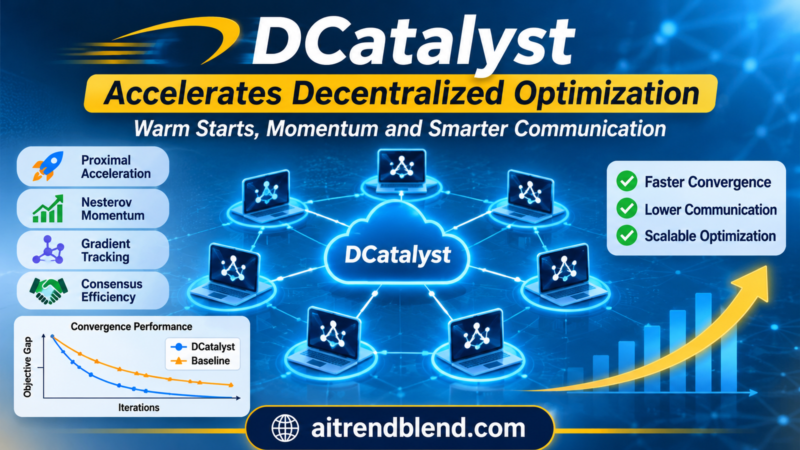
A group of machines trains one model while each machine keeps its own observations. There is no server collecting every update. Instead, neighbors exchange estimates and gradually agree. The local gradients may be cheap, yet the conversation takes a long time. DCatalyst asks whether an existing decentralized solver can keep its local machinery and still reduce the communication needed to reach an accurate solution.
- DCatalyst adds an accelerated proximal outer loop around a qualifying decentralized inner optimizer.
- The framework covers convex composite objectives, including a smooth loss plus a nonsmooth regularizer.
- Its guarantees depend on inner convergence, controlled subproblem error and a suitable warm start of auxiliary state.
- Similarity between local losses can improve communication bounds through a parameter describing differences in curvature.
- The experiments separate communication rounds from local gradient work and show a meaningful tradeoff between them.
- The reference implements the strongly convex linear SONATA specialization and discloses the limits of its practical inner budget.
An acceleration wrapper for a network of local solvers
Tianyu Cao, Xiaokai Chen and Gesualdo Scutari of Purdue University develop the framework in DCatalyst, published in the Journal of Machine Learning Research. Their setting is a fixed, connected and undirected network. Each agent knows its own smooth loss, while all agents share the same convex regularizer and seek the same solution.
The contribution is a reusable acceleration framework and its analysis. It specializes to methods with different local updates, tracking variables and finite sum structures. This matters because a successful acceleration proof for one algorithm does not automatically transfer when a regularizer or a different communication protocol is introduced.
The idea follows the broader Catalyst approach of solving a sequence of regularized subproblems. Nesterov inspired momentum acts between those solves. In a network, however, each agent has a different approximate iterate and a different momentum center. The analysis must account for those disagreements as well as incomplete local optimization.
This places the work in Optimization & Learning Theory. The question is how quickly a specified convex objective can be solved over a network. The reported gains concern optimization effort, with communication and computation tracked as separate resources.
The objective couples private losses through one shared decision
The target is the average of the agents’ losses plus a proper, closed and convex regularizer. The regularizer may be nonsmooth or take an infinite value to enforce a constraint. The smooth average may be strongly convex, or merely convex. These cases lead to different convergence statements.
Every agent maintains its own copy of the decision variable. The copies must approach both agreement and an optimum of the shared objective. Agreement alone is insufficient. A network can reach consensus on a poor point if it mixes estimates without correctly representing the collective loss.
The assumptions specify differentiable convex local losses with bounded smoothness constants. The common regularizer permits familiar structures such as an absolute value penalty for sparsity. The paper’s elastic net logistic regression example combines this penalty with a quadratic term in the smooth loss.
Keeping data at an agent and exchanging model related quantities describes the optimization protocol. It does not establish a differential privacy guarantee or a secure communication mechanism. Likewise, the static undirected graph assumption is a concrete part of the analysis. Intermittent participation, directed links and asynchronous execution would require additional arguments.
Three condition numbers describe different difficulties
The paper distinguishes the conditioning of the global average from the worst conditioning of individual agents. A local objective can be poorly conditioned even when complementary information across agents makes the global objective well conditioned. An algorithm whose rate depends on the local condition number can therefore miss a collective advantage.
The finite sum case introduces another quantity. When an agent’s loss averages many sample losses, the average of their smoothness constants can exceed the smoothness of the local average. The stochastic condition number reflects the cost of algorithms that use individual sample gradients.
These quantities should not be substituted for each other when comparing methods. The paper explicitly notes that some existing smooth variance reduction methods have more favorable dependence on a different condition number, while the new specialization accommodates a composite objective. A rate with broader applicability can have a different dependence on the problem’s constants.
Network connectivity contributes its own difficulty. With a doubly stochastic gossip matrix, the quantity \(\rho=\|W-\mathbf1\mathbf1^{\mathsf T}/m\|\) measures how far one mixing step remains from perfect averaging. A small spectral gap means that information travels slowly. Adding outer momentum does not remove this network dependence.
Each outer step creates a better conditioned subproblem
At outer iteration \(k\), agent \(i\) adds a quadratic penalty centered at its current extrapolated point. The inner decentralized algorithm approximately solves the average of these modified local objectives. The regularizer remains part of the subproblem.
The extra curvature makes the inner task more strongly convex. A larger proximal coefficient can make that task easier relative to its conditioning, but it also changes how many outer steps are needed. Selecting the coefficient balances those two costs. It is not a free acceleration knob that should always be made as large as possible.
After the inner solve, each agent extrapolates using its new and previous decision estimates. For a strongly convex objective, the paper uses a constant acceleration parameter determined by the strong convexity and proximal coefficient. The resulting momentum coefficient has the familiar fractional form.
The minimizer of the averaged proximal problem depends on the average center, but agents do not need a server to form it explicitly. Their inner decentralized method works with their local centers. Disagreement between those centers is part of the approximation that the analysis must control.
The nearby analysis of block Riemannian majorization minimization also emphasizes the cost of inexact subproblems. The settings and targets differ. Here convexity supports convergence to an optimum, while the manifold framework discusses stationarity under its own assumptions. A shared proximal motif does not transfer one theorem into the other.
The inner method must satisfy a contract
The framework accepts an inner algorithm with a merit function that contracts linearly on strongly convex instances. The merit must also control the agents’ average squared distance to the common optimizer. This can include optimization error, consensus error and error in auxiliary tracking variables.
That contract gives the wrapper something stronger than a decreasing local loss. The state contains the agents’ estimates and whatever additional variables the inner method uses. Gradient trackers and dual variables can retain information essential to convergence even when the visible decision estimates look nearly identical.
For the strongly convex outer problem, the inner accuracy budget decreases geometrically. Under the prescribed warm start conditions, the analysis bounds the required inner work uniformly across outer iterations, with constants depending on the chosen method and proximal coefficient.
A small fixed number of inner iterations does not by itself establish this inequality. The experiment’s convenient schedule and the theorem’s sufficient error control play different roles. Implementations should record which one they use, rather than treating any capped inner solve as certified.
“inexact solutions of local subproblems”Cao, Chen and Scutari, describing the errors their estimating sequence analysis accommodates.
An outer acceleration formula is only one part of the method. The inner contraction, the accuracy schedule and the state carried into the next subproblem determine whether the accelerated argument applies.
Warm starts preserve more than the model weights
The next inner problem begins near the previous solution, so restarting the decision variable from zero would waste useful progress. The auxiliary state also needs a deliberate transition. The paper’s warm start assumption bounds the new initial merit by the old final merit plus a term measuring movement in the centers.
For a gradient tracking method, changing the proximal center changes the local objective gradient even when the decision variable stays fixed. A tracker that still represents the old objective is therefore stale at the start of the new solve. Its correction can be computed locally from the center movement.
This identity reveals a sign discrepancy in the source. Equation 13 prints a tracker restart with the new center minus the old center. Differentiating the subproblem in equation 5 gives the reverse order above, and the appendix calculation in equation 47 uses the old center minus the new center. The reference follows the explicit gradient difference. This is a disclosed interpretation of the displayed formulas, rather than a claim to have inspected an authors’ code release.
The invariant worth checking is simple. With doubly stochastic mixing and correct initialization, the average tracker should match the average current local gradient. The correction must preserve that identity after recentering. This numerical check can catch a restart error before a long experiment produces an attractive but misleading curve.
Other decentralized methods carry different state and need different warm starts. The paper develops these conditions for SONATA, PUDA and a variance reduction method. Our article on constrained stochastic optimization provides a neighboring example of why auxiliary variables belong in a method description, although its inference results do not establish the acceleration guarantee here.
Similarity can reduce the communication burden
The paper’s similarity condition concerns how differences between local and global gradients change as the decision variable moves. For twice differentiable objectives, this can be understood through closeness between local and global curvature. A small value can coexist with a substantial difference between gradients at a particular point.
SONATA offers two relevant surrogate choices. The linear variant uses first order information and a quadratic term, usually leading to an easy proximal update. The full function variant retains the local loss and adds a movement penalty. That richer local problem can exploit similarity but can cost more to solve.
For the strongly convex case, the selected communication bounds show the difference. The linear specialization depends on the global condition number. The similarity aware specialization can replace that dependence with the smaller similarity ratio when the assumptions and tuning hold.
The notation hides specified logarithmic factors in problem parameters. It does not erase every dependence on the target accuracy. The computation bounds for the two methods also differ, including the work needed for local subproblem solves. A smaller communication expression alone is insufficient to predict elapsed time.
Similarity is a structural opportunity, not an automatic consequence of distributing data. Independent samples from a common distribution can support favorable similarity bounds under further conditions. A partition with very different local curvature may provide much less benefit. The measured or justified similarity parameter should accompany the claim.
Convex and finite sum extensions require their own metrics
When strong convexity is absent, the momentum parameter changes across outer steps. The prescribed inner accuracy decays polynomially, and the analysis bounds the inner iteration growth logarithmically under additional conditions, including bounded iterates. This is a different regime from the constant parameter strongly convex construction.
The general convex outer statement uses the gradient of the Moreau envelope as its accuracy measure. In smooth special cases, the paper also bounds the objective gradient. An accelerated rate for that measure should not be rewritten without explanation as the same rate for every objective gap or every agent’s model error.
For finite sum losses, the paper wraps PMGT with loopless variance reduced gradients. Under the stated setup, the accelerated specialization reaches a communication dependence involving the square root of the product of local sample size and stochastic condition number, together with the network term.
The attractive regime is an ill conditioned problem in which variance reduction and acceleration can save meaningful work. The paper also acknowledges stronger condition number dependence for some existing smooth methods. Its composite extension is part of the contribution, so comparisons should retain the regularizer and the applicable function class.
What the experiments measure
The default network has thirty agents connected through a random undirected graph with edge probability 0.5. Algorithms use Metropolis style gossip weights. These are simulated network experiments. Their communication axis counts rounds of exchange, while their computation axis counts the specified optimization or gradient work.
The distinction extends to the reported error. In strongly convex experiments, the gap is average squared distance between the agents’ estimates and the optimizer. In merely convex experiments, the plotted gap is an average objective difference. Neither quantity is classification accuracy on unseen images.
The main elastic net example uses MNIST from LIBSVM, with 60,000 observations and 784 features. The local objective is binary logistic loss plus a quadratic penalty, with an absolute value regularizer shared across agents. The stated model therefore requires an explicit binary label construction in any reproduction.
For the first strongly convex comparison, the paper uses an absolute value coefficient of 0.01 and a quadratic coefficient of 0.5. The reported global condition number is twenty and the similarity ratio is 3.1. This is a setting where exploiting similarity should help. The full function SONATA specialization performs particularly well, while the linear specialization reduces communication relative to DPAG with comparable iteration work.
| Experiment | Reported setting | Observed comparison | Interpretation |
|---|---|---|---|
| Strongly convex elastic net logistic regression | 30 agents, 60,000 observations, 784 features, similarity ratio 3.1 | The similarity aware specialization gains most when local functions are similar | Compare communications and local work separately |
| Convex logistic regression with absolute value penalty | No quadratic term and penalty coefficient \(10^{-4}\) | The linear DCatalyst specialization improves on APM in the displayed curves | The plot uses objective gap rather than the strongly convex distance metric |
| Composite finite sum logistic regression | 6,000 MNIST observations, 200 per agent, \(\kappa_s\approx2.73\times10^5\) | Wrapping PMGT with acceleration reduces both displayed resource costs | The experiment targets a large stochastic condition number |
| Smooth ridge regression with variance reduction | Batch sizes one, one hundred and one thousand | Larger batches reduce communication while increasing gradient work | A communication saving can accompany a computation increase |
The similarity experiment varies local sample size and quadratic regularization to study the roles of conditioning and similarity. It measures the communication needed to reduce the strongly convex gap below \(10^{-4}\). The trends support the predicted dependence, while the experimental construction does not provide a universal ranking for arbitrary partitions.
The finite sum logistic experiment uses absolute value coefficient \(10^{-7}\) and quadratic coefficient \(10^{-4}\). Its local sample count of two hundred is much smaller than the reported stochastic condition number. This deliberately emphasizes a regime where the accelerated variance reduction argument should be useful.
The ridge experiment adds another practical lesson. Increasing the batch can improve the communication curve while worsening the computation curve. The paper does not supply a general wall clock speedup that combines those resources. Hardware, message size, parallelism and the relative price of local gradients would be needed to make that claim.
The additional smooth convex experiment also prevents an overly broad conclusion. The linear DCatalyst specialization uses fewer communications than its comparators there, but loses some computational ground to APM with consensus. The paper attributes this to additional logarithmic factors. A fair account retains that tradeoff alongside the favorable main results.
Pick a resource model before declaring a winner. Count every gossip operation, include local solver work, and state the accuracy metric. A faster communication curve answers a different practical question from lower gradient cost or shorter elapsed time.
Limits to check before wrapping a new optimizer
The inner algorithm needs the required merit contraction on the regularized subproblems and a compatible warm start. Matching the outer update while replacing the inner method with an arbitrary optimizer leaves those requirements unresolved. This is especially relevant when an inner method carries a gradient estimate or dual state.
The theory concerns convex losses and convex regularization. It does not certify acceleration of a general deep neural network training problem. Our article on bilevel saddle point avoidance concerns different assumptions and a different optimality target. Those distinctions remain important even when both algorithms contain nested loops.
Problem constants influence practical tuning. Strong convexity, smoothness, graph contraction and similarity may be known only through bounds. Conservative values can increase communication substantially. Loose constants and a difficult local solve can offset the apparent simplicity of the wrapper.
Network and data variations also matter. The experimental default is a reasonably dense random graph. A sparse graph, failures or delayed messages can change the relative cost of consensus. A source gradient calculation designed for one stochastic setting should not be assumed valid under temporally dependent observations. The discussion of stochastic approximation with dependent noise offers adjacent context, without extending DCatalyst’s theorem to that setting.
The remaining logarithmic factors are an acknowledged limitation. The authors identify a possible unified single loop design as a future direction. That leaves room for improved theory and implementations while preserving the paper’s contribution to composite decentralized acceleration.
A reusable wrapper needs an explicit inner contract
DCatalyst provides a common route to accelerate several decentralized optimization methods. Its strength is the combination of modular algorithm design with a proof mechanism that can represent consensus error and incomplete subproblem solves. That is more reusable than a momentum formula considered in isolation.
The conceptual shift is to treat the network’s error as part of the approximation budget. Each agent’s decision, momentum center and auxiliary state contribute to the trajectory. A valid wrapper must carry these relationships across successive proximal subproblems.
The framework is especially appealing when communication is expensive, the objective is ill conditioned and the local update structure can be reused. Similar local curvature can improve the communication dependence further, provided the selected inner method is designed to exploit it. Finite sum structure supplies another opportunity through variance reduction.
The practical limits are equally concrete. Suitable inner accuracy, valid restart formulas and credible problem constants remain necessary. The reported optimization gains do not establish improved test accuracy, automatic privacy or a universal wall clock advantage across networks.
A useful next evaluation would report the same optimization target against communication rounds, gradient work, bytes exchanged and elapsed time on the intended topology. That would connect the framework’s resource bounds to deployment decisions. The immediate lesson is to choose the inner solver and the communication budget together.
Complete PyTorch reference for the linear SONATA specialization
The listing implements elastic net binary logistic regression, analytic local gradients, a connected random graph, Metropolis weights, the linear SONATA update, gradient tracking, outer proximal acceleration and warm restarts. It includes model and state classes, the loss and proximal operation, fitting loops, evaluation, a plain solver baseline and a runnable synthetic smoke test.
All agents run in one process for clarity. Each update uses its local gradient and neighbor mixing operations. The simulator computes shared curvature bounds and diagnostics from its stored data. It is not a transport layer, a privacy mechanism, a variance reduction implementation or a reproduction of the MNIST figures.
Repeated gossip is counted explicitly and chosen conservatively to satisfy the stated sufficient mixing bound for the linear inner method. The outer routine uses a fixed inner iteration schedule resembling the reported experiment. It does not verify the paper’s merit accuracy budget and marks that limitation in its returned settings. The numerical central reference and global diagnostics never determine agent updates or stopping budgets.
Communication counts use two mixing phases per inner step, each with its repeated graph operations. Diagnostic costs are excluded and labeled accordingly. The smoke test checks tracker consistency, dimensions and finite numerical behavior rather than asserting a speedup. Python syntax and independent NumPy checks of gradients, the proximal update, mixing and recentering passed. PyTorch is unavailable here, so the included runtime smoke test has not been executed.
"""Editorial DCatalyst/SONATA-L reference for Cao et al., JMLR 27(47), 2026.

Requires Python 3.10+ and PyTorch. Run for a small synthetic smoke test.
Strongly convex elastic-net binary logistic regression, CPU float64.
All agents are simulated in one process. No socket transport, privacy protocol,
SONATA-F, PUDA, variance reduction or MNIST benchmark is implemented.
The deterministic inner budget illustrates the experiment's log-condition
schedule. It does NOT certify the paper's merit-function stopping condition.
Global evaluations and a central reference are diagnostics, never agent updates.
"""
from dataclasses import dataclass
import math
import torch
from torch import nn
from torch.nn import functional as F

DTYPE = torch.float64


def soft_threshold(x, threshold):
    return torch.sign(x)*torch.clamp(torch.abs(x)-threshold,min=0)


class PeerLogisticModel(nn.Module):
    def __init__(self, features, labels, ridge=.2, lasso=.01):
        super().__init__()
        features = torch.as_tensor(features,dtype=DTYPE,device="cpu")
        labels = torch.as_tensor(labels,dtype=DTYPE,device="cpu")
        if features.ndim != 3 or labels.shape != features.shape[:2]:
            raise ValueError("Need features [agents,samples,dimension] and labels [agents,samples].")
        if features.shape[0] < 2 or min(features.shape[1:]) < 1:
            raise ValueError("Need multiple agents, samples and feature coordinates.")
        if not torch.isfinite(features).all() or not torch.isfinite(labels).all():
            raise ValueError("Data must be finite.")
        if not ((labels == -1) | (labels == 1)).all() or ridge <= 0 or lasso < 0:
            raise ValueError("Use binary +/-1 labels, positive ridge and nonnegative lasso.")
        self.register_buffer("features",features)
        self.register_buffer("labels",labels)
        self.ridge, self.lasso = ridge, lasso
        self.agents,self.samples,self.dimension = features.shape
        # Logistic Hessian is bounded by A.T A/(4n) + ridge*I.
        bounds = torch.einsum("mnd,mne->mde",features,features)/(4*self.samples)
        bounds += ridge*torch.eye(self.dimension,dtype=DTYPE)
        self.Lmax = float(torch.linalg.eigvalsh(bounds).max())
        self.L = float(torch.linalg.eigvalsh(bounds.mean(0)).max())
        self.mu = ridge  # Conservative common strong-convexity lower bound.

    def forward(self, weights):
        return torch.einsum("mnd,md->mn",self.features,weights)

    def local_gradient(self, weights):
        scores = self(weights)
        multipliers = -self.labels*torch.sigmoid(-self.labels*scores)
        return (torch.einsum("mnd,mn->md",self.features,multipliers)/self.samples
                + self.ridge*weights)

    def global_gradient(self, weight):
        # Diagnostic/global reference only, not a message in the peer algorithm.
        repeated = weight.expand(self.agents,-1)
        return self.local_gradient(repeated).mean(0)

    def objective(self, weight):
        scores = torch.einsum("mnd,d->mn",self.features,weight)
        return (F.softplus(-self.labels*scores).mean()
                + self.ridge*weight.square().sum()/2
                + self.lasso*weight.abs().sum())


def metropolis_graph(agents, probability=.5, seed=0):
    """Rejection-sample a connected undirected Erdos-Renyi graph."""
    if agents < 2 or not 0 < probability <= 1:
        raise ValueError("Need multiple agents and a valid edge probability.")
    generator = torch.Generator().manual_seed(seed)
    for _ in range(200):
        upper = torch.triu(torch.rand(agents,agents,generator=generator)<probability,diagonal=1)
        adjacency = upper | upper.T
        seen, frontier = {0}, [0]
        while frontier:
            node = frontier.pop()
            for neighbor in torch.where(adjacency[node])[0].tolist():
                if neighbor not in seen:
                    seen.add(neighbor)
                    frontier.append(neighbor)
        if len(seen) == agents:
            break
    else:
        raise RuntimeError("Could not sample a connected graph.")
    degree = adjacency.sum(1)
    weights = torch.zeros(agents,agents,dtype=DTYPE)
    for i in range(agents):
        for j in torch.where(adjacency[i])[0].tolist():
            weights[i,j] = 1/(1+max(int(degree[i]),int(degree[j])))
        weights[i,i] = 1-weights[i].sum()
    return weights


def mixing_budget(weights, mu, L, Lmax):
    """Power the gossip map to meet the sufficient SONATA-L bound in Lemma 7.

    Every application still uses the original neighbor graph and is counted.
    This conservative construction is not a tuned speed benchmark.
    """
    agents = len(weights)
    average = torch.ones_like(weights)/agents
    rho = float(torch.linalg.matrix_norm(weights-average,ord=2))
    if rho >= 1:
        raise ValueError("The graph must mix.")
    target_squared = min(mu**2/(13440*Lmax**2),L**2/(12*L**2+84*Lmax**2))
    target = math.sqrt(target_squared)
    rounds = 1 if rho < 1e-14 else max(1,math.ceil(math.log(target)/math.log(rho)))
    return rounds,rho


@dataclass
class SolverState:
    x: torch.Tensor
    tracker: torch.Tensor
    gradient: torch.Tensor


class SONATAL:
    def __init__(self,model,weights,delta=0.):
        weights = torch.as_tensor(weights,dtype=DTYPE,device="cpu")
        if weights.shape != (model.agents,model.agents) or (weights < 0).any():
            raise ValueError("Invalid gossip weight matrix.")
        if not torch.allclose(weights,weights.T) or not torch.allclose(
                weights.sum(0),torch.ones(model.agents,dtype=DTYPE)):
            raise ValueError("Use symmetric doubly stochastic weights.")
        self.model,self.weights,self.delta = model,weights,delta
        self.tau = model.L+delta
        self.rounds,self.rho = mixing_budget(
            weights,model.mu+delta,model.L+delta,model.Lmax+delta)
        self.communication_rounds = 0
        self.gradient_calls_per_agent = 1

    def mix(self,values):
        for _ in range(self.rounds):
            values = self.weights@values
            self.communication_rounds += 1
        return values

    def initialize(self):
        x = torch.zeros(self.model.agents,self.model.dimension,dtype=DTYPE)
        z = x.clone()
        gradient = self.model.local_gradient(x)+self.delta*(x-z)
        return SolverState(x,gradient.clone(),gradient),z

    @torch.no_grad()
    def step(self,state,centers):
        # Linear surrogate: local gradient terms cancel the tracker correction.
        half = soft_threshold(state.x-state.tracker/self.tau,
                              self.model.lasso/self.tau)
        new_x = self.mix(half)
        gradient = self.model.local_gradient(new_x)+self.delta*(new_x-centers)
        self.gradient_calls_per_agent += 1
        # Mix the complete tracker-plus-gradient-difference expression.
        tracker = self.mix(state.tracker+gradient-state.gradient)
        return SolverState(new_x,tracker,gradient)

    @torch.no_grad()
    def recenter(self,state,old_centers,new_centers):
        # grad[fi + delta/2 ||x-z||^2] changes by delta*(z_old-z_new).
        # Equation (13) prints the opposite sign; Appendix (47) uses this order.
        change = self.delta*(old_centers-new_centers)
        return SolverState(state.x,state.tracker+change,state.gradient+change)


@torch.no_grad()
def evaluate(model,state,centers,delta,reference=None):
    average = state.x.mean(0)
    gradient = model.global_gradient(average)
    proximal = soft_threshold(average-gradient/model.L,model.lasso/model.L)
    current = model.local_gradient(state.x)+delta*(state.x-centers)
    metrics = {
        "objective_at_average":float(model.objective(average)),
        "consensus_error":float((state.x-average).square().sum(1).mean()),
        "proximal_gradient_norm":float(model.L*torch.linalg.vector_norm(average-proximal)),
        "tracker_mean_error":float(torch.linalg.vector_norm(state.tracker.mean(0)-current.mean(0))),
    }
    if reference is not None:
        metrics["mean_squared_distance_to_reference"] = float(
            (state.x-reference).square().sum(1).mean())
    return metrics


@torch.no_grad()
def central_reference(model,tolerance=1e-9,max_steps=50000):
    """Numerical reference only. Never used by decentralized updates or budgets."""
    x = torch.zeros(model.dimension,dtype=DTYPE)
    for _ in range(max_steps):
        new_x = soft_threshold(x-model.global_gradient(x)/model.L,model.lasso/model.L)
        residual = float(model.L*torch.linalg.vector_norm(new_x-x))
        x = new_x
        if residual < tolerance:
            return x
    raise RuntimeError("Central reference did not meet its numerical tolerance.")


@torch.no_grad()
def fit_dcatalyst(model,weights,outer_steps=30,inner_steps=None,reference=None):
    delta = max(model.L-model.mu,model.mu*1e-6)
    alpha = math.sqrt(model.mu/(model.mu+delta))
    momentum = (1-alpha)/(1+alpha)
    if inner_steps is None:
        inner_steps = max(1,math.ceil(math.log(model.L/model.mu)))
    if outer_steps < 1 or inner_steps < 1:
        raise ValueError("Use positive iteration budgets.")
    solver = SONATAL(model,weights,delta)
    state,centers = solver.initialize()
    history = []
    for outer in range(outer_steps):
        previous = state.x.clone()
        for _ in range(inner_steps):
            state = solver.step(state,centers)
        new_centers = state.x+momentum*(state.x-previous)
        state = solver.recenter(state,centers,new_centers)
        centers = new_centers
        metrics = evaluate(model,state,centers,delta,reference)
        metrics.update(outer=outer+1,communication_rounds=solver.communication_rounds,
                       sample_gradients_per_agent=solver.gradient_calls_per_agent*model.samples)
        history.append(metrics)
    return state,history,{"delta":delta,"alpha":alpha,"mixes_per_phase":solver.rounds,
                          "inner_steps":inner_steps,"paper_accuracy_verified":False,
                          "diagnostic_costs_excluded":True}


@torch.no_grad()
def fit_plain(model,weights,steps=60,reference=None):
    solver = SONATAL(model,weights)
    state,centers = solver.initialize()
    history = []
    for step in range(steps):
        state = solver.step(state,centers)
        metrics = evaluate(model,state,centers,0.,reference)
        metrics.update(step=step+1,communication_rounds=solver.communication_rounds,
                       sample_gradients_per_agent=solver.gradient_calls_per_agent*model.samples)
        history.append(metrics)
    return state,history


def synthetic_data(agents=6,samples=40,dimension=8,seed=2):
    """Own binary logistic example. No undocumented MNIST label mapping."""
    generator = torch.Generator().manual_seed(seed)
    features = torch.randn(agents,samples,dimension,generator=generator,dtype=DTYPE)
    truth = torch.linspace(-.5,.5,dimension,dtype=DTYPE)
    probability = torch.sigmoid(torch.einsum("mnd,d->mn",features,truth))
    labels = 2*torch.bernoulli(probability,generator=generator)-1
    return features,labels


def smoke_test():
    torch.set_num_threads(2)
    features,labels = synthetic_data()
    model = PeerLogisticModel(features,labels)
    weights = metropolis_graph(model.agents,seed=4)
    torch.testing.assert_close(weights,weights.T)
    torch.testing.assert_close(weights.sum(0),torch.ones(model.agents,dtype=DTYPE))
    reference = central_reference(model)
    state,history,settings = fit_dcatalyst(model,weights,outer_steps=12,reference=reference)
    _,plain = fit_plain(model,weights,steps=24,reference=reference)
    assert all(math.isfinite(v) for row in history for v in row.values())
    assert history[-1]["tracker_mean_error"] < 1e-8
    assert history[-1]["objective_at_average"] < float(model.objective(torch.zeros(model.dimension,dtype=DTYPE)))
    # A wrong warm-restart sign breaks this invariant even before convergence.
    assert state.x.shape == (model.agents,model.dimension)
    print("DCatalyst reference",history[-1],settings)
    print("Plain SONATA-L reference",plain[-1])
    print("No MNIST reproduction or merit-budget certificate is claimed.")


if __name__ == "__main__":
    smoke_test()
Frequently asked questions
What does DCatalyst accelerate?
It accelerates qualifying decentralized methods for convex composite objectives by wrapping them in an inexact proximal scheme with momentum. The inner method must satisfy the required convergence and warm start conditions.
Does DCatalyst need a central server?
The optimization framework uses neighbor communication on a fixed connected undirected graph. The editorial code simulates those agents in one process and uses global calculations only for tuning bounds and diagnostics.
Why do communication and computation results differ?
A local solver or a larger batch can reduce the number of exchanges while increasing local gradient work. The paper reports these resources separately, so a communication improvement alone does not establish an elapsed time speedup.
What does similarity between local functions mean?
It bounds how the difference between a local gradient and the global gradient changes between two points. It is related to curvature similarity and does not require local gradients to be equal at a given point.
Can the convex theory be applied directly to a deep network?
No. The results require the stated convexity, smoothness, network and inner solver assumptions. They do not certify general acceleration of nonconvex neural network training.
Has the reference reproduced the paper’s experiments?
No. The code implements a complete strongly convex linear SONATA specialization with synthetic data. Syntax and independent numerical checks passed, but PyTorch runtime testing was unavailable and the fixed inner budget is not a merit accuracy certificate.
Read the paper and inspect the reference
The publisher provides the full paper and bibliographic record. Its page does not list an authors’ code repository. The download below is the complete editorial reference printed in this article.
Read the JMLR paperDownload editorial referenceTianyu Cao, Xiaokai Chen and Gesualdo Scutari. DCatalyst. A Unified Accelerated Framework for Decentralized Optimization. Journal of Machine Learning Research, volume 27, article 47, pages 1 to 57, 2026. Algorithms 1 and 2, Assumptions 1 to 5, Theorems 3 and 6, Corollaries 9, 10 and 17, Section 7 and Appendix B provide the principal evidence discussed here.
This analysis is based on the published paper and an independent evaluation of its claims.