
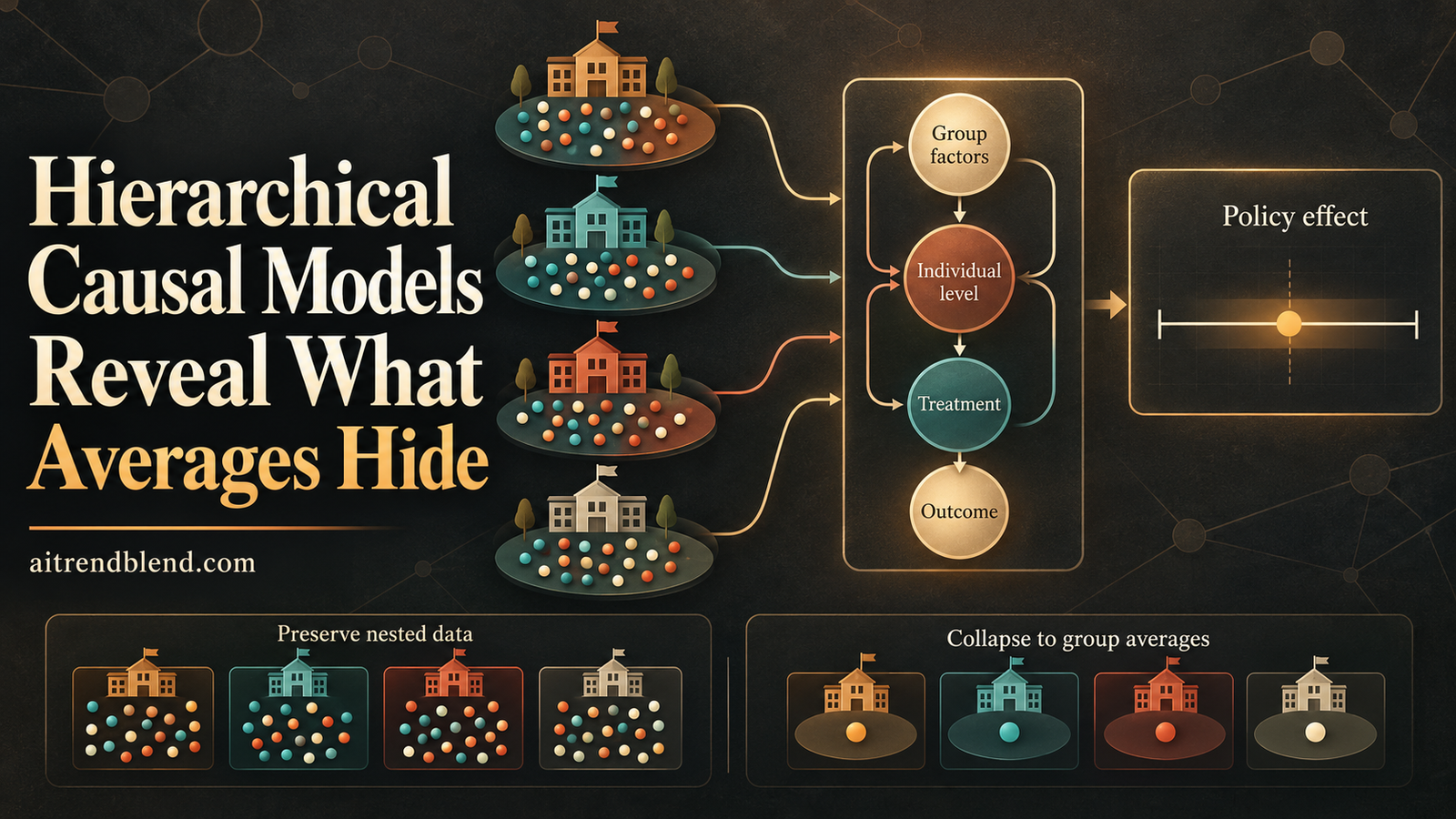
A school offers a test preparation program. Some students attend, others do not, and the analyst records their results. Now imagine the school doubles enrollment. The program changes for the newly enrolled students, but it may also change for everyone already attending because classes become larger. A model that estimates the benefit of attending under the original conditions has not automatically answered what happens when the program expands. Hierarchical causal models make that difference visible.
Key points
- Hierarchical causal models describe causes among subunits within units, including paths that leave a group of subunits and return through a shared variable.
- The framework retains distributions within groups rather than assuming group averages contain everything needed for causal inference.
- Hidden group confounding can be addressed in some graphs, but hidden confounding among individuals remains a separate threat.
- The identification results require infinitely many subunits and mechanisms that converge in that limit. Finite datasets need additional estimation choices.
- In the eight schools analysis, allowing interference changes the posterior mean only slightly but greatly widens posterior uncertainty.
- The reference code implements the paper’s binary unit confounder example. The authors’ repository supplies the broader experiments.
Research context
This article explains published research and is not medical advice, diagnosis or treatment. Consult a qualified professional about health decisions. The paper mentions possible biological applications but reports no patient study, diagnostic evaluation or clinical treatment validation. No medical reviewer has been supplied.
Why a good prediction does not answer a policy question
Suppose an analyst predicts scores accurately from attendance and school identity. That achievement says the model has learned something useful about the observed data. It does not establish the result of changing attendance. A prediction describes how variables occur together under existing conditions. A causal intervention asks what happens when part of the process producing those variables is replaced.
Nested data complicates this distinction because the process has several levels. Students share resources within a school. Customers share an online marketplace. Individual observations can influence a shared condition that subsequently affects other observations. Removing those levels before analysis can erase the difference between an individual response and a response to a collective change.
Eli N. Weinstein of the Technical University of Denmark and David M. Blei of Columbia University develop this problem in Hierarchical Causal Models, published in the Journal of Machine Learning Research in January 2026. Their contribution is a framework for deciding when a causal question is identifiable from nested observational information. It is not a classifier architecture or a method that automatically discovers the correct graph.
That distinction shapes how to read the paper. Identification means an effect is determined by the observational distribution together with stated causal assumptions. Estimation means approximating that effect from a finite sample. An optimizer may solve the estimation problem efficiently while the identification problem remains impossible. Related questions about estimation uncertainty appear in our article on statistical inference in constrained optimization. More training cannot replace a missing causal assumption.
This analysis belongs in the site’s Machine Learning category because it addresses how data structure changes what can be learned about interventions. Its practical angle is a modeling audit. Before fitting a predictor, decide whether the intervention acts on an individual, a whole group, or the distribution of individual actions within a group.
The information hidden inside a group
A school average can hide several different populations. Two schools can have similar average participation and average performance while differing in who participates, how outcomes vary with participation, and how students interact through school resources. Keeping individual records allows an analyst to estimate relationships within each school instead of relying only on relationships between schools.
The authors formalize this using units and subunits. Index \(i\) names a unit and \(j\) names a subunit within it. A variable such as school budget has one value per unit. A variable such as student attendance has one value per subunit. The graph marks this distinction with an inner plate for repeated subunit observations inside an outer plate for repeated units.
Plates are familiar in probabilistic modeling, but their causal interpretation needs care. A subunit variable may depend on its own subunit parents and on shared unit parents. A unit variable can depend on the collection of subunit parents. That collection must be treated without privileging an arbitrary ordering of subunits. Changing the order of student records should not change the school mechanism.
A representative structural equation from the paper. Shared unit causes and unit noise affect every subunit, while individual treatment and individual noise affect the corresponding observation.
The shared noise is more than a device for correlated errors. It can represent a hidden cause of both treatment assignment patterns and outcomes across schools. If a better resourced school can offer more places and more effective teaching, participation and scores may rise together even if attending contributes less than the association suggests.
The model assumes units are exchangeable and subunits are exchangeable within units. This does not mean all groups have identical effects. It means their generation can be represented through shared population mechanisms rather than through a special causal role for a record’s index. Nearby points in time or space may violate this assumption. A patient trajectory or a spatial network cannot be made exchangeable merely by placing it in a table.
Weinstein and Blei connect their framework to structural causal models associated with Pearl, hierarchical Bayesian models discussed by Gelman and colleagues, and established methods for effects within groups. These are references discussed in the supplied paper. The new organizing idea is to make causal reasoning operate on nested distributions and shared mechanisms, rather than treating hierarchy as only a correlation problem.
Three graphs that require three different answers
Hidden unit confounding
In the first motif, an unobserved unit variable influences individual treatment and individual outcome, with a direct arrow from treatment to outcome. There is no hidden individual confounder in this example and no path through a shared consequence of treatment. The hidden unit cause stays fixed when comparing subunits inside the same unit.
This structure motivates estimating the outcome relationship separately within each unit and then averaging the resulting intervention means across units. It recovers a familiar justification for methods that control for group differences, including appropriate regression methods with group effects. The paper is explicit that its first example connects to existing techniques rather than replacing them with a wholly new estimator.
However, saying that a group label controls for confounding is a statement about this graph. It is not a universal license to interpret any coefficient from a model containing school identifiers as causal. If individual motivation affects both attendance and scores, for example, a school indicator cannot absorb that individual source of confounding.
Confounding with interference
The second motif introduces a unit variable influenced by subunit treatments that subsequently influences subunit outcomes. Think of attendance affecting shared class size, which affects performance. The outcome mechanism can now change when the intervention changes the treatment distribution in a school.
An estimate that holds class size at its observed value answers a different question from an estimate that lets class size respond to expanded attendance. This is where treating school identity as a dummy variable becomes insufficient. It can account for a persistent school difference, but it does not describe how the school changes in response to the proposed policy.
The paper derives a correction using the observed shared intermediary and distributional variables. Its graphical reasoning resembles a front door adjustment after the appropriate transformation of the hierarchical graph. The observed intermediary must support that reasoning. An unobserved or incorrectly modeled interference route is not repaired by calling the model hierarchical.
A subunit instrument with a unit outcome
In the third motif, the outcome is measured for the unit, while a subunit instrument influences subunit treatment. The instrument has no parents and treatment is its only child in the stated graph. Variation in the instrument helps reveal treatment assignment mechanisms within a unit, even though the outcome is observed at a different level.
The analysis retains the conditional distribution of treatment given the instrument within each unit. It uses that distribution to adjust the population relationship between the marginal treatment distribution and the unit outcome. The key is the assumed instrument structure, plus the support required for the intervention. Any variable correlated with treatment cannot simply be declared an instrument.
| Motif | Observed information that matters | Main danger of simplification |
|---|---|---|
| Unit confounder | Outcome given treatment within each unit | Regression on group averages can mistake group confounding for an individual effect |
| Unit confounder with interference | Treatment distributions, outcome conditionals and the shared intermediary | Holding the observed intermediary fixed misses its response to intervention |
| Subunit instrument | Treatment given instrument within units and the unit outcome | Ignoring instrument information leaves the aggregate relationship confounded |
Key takeaway
The correct adjustment follows the causal graph. Group identity can address a shared confounder in one graph and fail to represent interference in another.
Turning a collection of records into a causal variable
The paper’s identification workflow has four stages. Collapse the hierarchical model into a model containing distributions within units. Augment it with the distributional quantities needed for the intervention or outcome. Apply graphical identification tools, with marginalization when appropriate. Finally estimate the terms using the actual data.
Collapsing is the least intuitive step. A conditional distribution within a unit becomes a variable that changes from one unit to another. Instead of treating every student as a separate node in an enormous graph, the transformed graph contains objects such as a school’s treatment distribution and its conditional outcome distribution.
The capital symbols denote random distributions across units. The last expression constructs an outcome marginal from a treatment marginal and an outcome conditional.
These quantities are distributions, not just mean vectors. For a binary variable, one probability can describe a marginal, so the distinction is easy to overlook. For a continuous or structured variable, a mean may omit variance, tails or other features through which a shared mechanism operates. Replacing every distribution with its mean is an additional modeling decision.
Augmentation adds deterministic relationships such as the outcome marginal above. This lets an intervention on the treatment distribution be connected to a well defined outcome quantity. Deterministic nodes need special attention because naive density manipulations can create impossible conditioning events. The instrument example uses marginalization to obtain a suitable stochastic relationship and satisfy positivity requirements.
The collapse theorem relies on taking the number of subunits toward infinity and on mechanisms converging in that limit. A unit mechanism based on a stable empirical average is a natural example. A mechanism that oscillates as the number of subunits changes is not. Infinite subunits are therefore part of the identification argument, not an optional convenience inserted only for computation.
In an application, neither the empirical treatment distribution nor the conditional outcome model is known exactly. Both are estimated from finite observations. Errors from that first stage then enter the population stage. This creates a reason to measure data adequacy along two axes. More units improve learning about the population of groups. More subunits improve learning about each group’s internal mechanism.
Write the intervention before writing the estimator
A hard intervention sets treatment to a fixed value. A soft intervention draws treatment from a specified distribution, possibly conditional on allowed observed parents. For a binary treatment, a common soft policy uses a Bernoulli distribution with a chosen enrollment probability. Both kinds of intervention replace the treatment mechanism rather than merely conditioning on observed treatment.
The first policy sets treatment deterministically. The second sets a treatment probability. These are intervention definitions, not fitted propensities.
For the unit confounder motif, the intervention leaves the distribution of unit outcome conditionals unchanged. One can integrate the new treatment policy against each conditional response and average over units. Equations 23 and 24 in the paper give the following estimation logic.
This binary specialization averages units equally. Changing the target to an average across individuals would require an explicit weighting choice.
That weighting issue is easy to miss in an implementation. A large school does not receive more weight merely because it supplies more student records when the estimand averages the population of schools equally. If the policy target is a population of students instead, the analyst must specify how school sizes enter the target distribution. The code should follow that choice explicitly.
In the interference motif, the conditional outcome distribution itself responds through the shared intermediary. Equation 27 identifies its intervention distribution using the treatment distribution and the intermediary.
The outer term predicts how the shared intermediary responds to the policy. The inner adjustment averages outcome mechanisms over observed treatment distributions.
The formula is not a recommendation to adjust for every variable measured after treatment. Its validity follows from the stated graph and support assumptions. Adding or removing an arrow can change the identification argument. In particular, a hidden cause of the intermediary and outcome may destroy the route used by this motif.
For the subunit instrument example, Equation 31 uses the distribution of treatment given the instrument as the adjustment object.
The model must provide the required support for the proposed marginal treatment distribution within the relevant conditional mechanism strata.
This makes overlap a concrete question. Can the observed data support the policy being requested within the needed strata? A fitted regression can emit a number beyond observed support, but producing that number does not establish nonparametric identification. Model extrapolation and observational identification should be reported separately.
What the simulations demonstrate
The paper uses three simulation families corresponding to its central motifs. The true causal graph and data generating mechanisms are known by construction. That is useful for checking whether the identified formulas lead to the correct effect as data increase. It does not test whether an analyst can infer the true graph from an uncontrolled dataset.
For the unit confounder simulation, both the number of units and the number of subunits increase together. Appendix D.1 describes generating datasets with 1000 units and 1000 subunits per unit, then examining subsets. Figure 7 reports standard deviations across 20 independent simulations, with confounding settings of zero, 0.2 and 0.5.
The HCM estimator approaches the true effect in all three settings. The comparison regression predicts each unit’s average outcome from its average treatment. It approaches the truth without confounding but remains biased under confounding. This comparison illustrates lost identification information in the aggregate relationship. It does not show that every possible regression method fails.
Figure 8 considers shared interference strengths of zero, 0.5 and 1.5, again reporting variation over 20 simulations. The confounder estimator that omits interference becomes inadequate when interference is present, whereas the estimator derived for the full motif approaches the relevant asymptotic truth as data increase. The simulated ground truth has large finite groups, while the identifying formula uses the infinite subunit limit.
Figure 9 compares policies with Bernoulli probabilities of 0.75 and 0.25 in the instrument motif. The authors use Gaussian process classification rather than the correctly specified parametric models used in the earlier examples. Bias and variability are more visible. Their additional experiments show how increasing subunits relative to units can reduce bias at smaller unit counts.
| Source | Variation examined | Reported finding | What it does not establish |
|---|---|---|---|
| Figure 7 | Confounding settings 0, 0.2 and 0.5 | The nested estimator approaches truth while aggregate regression remains biased with confounding | Recovery under hidden individual confounding |
| Figure 8 | Interference strengths 0, 0.5 and 1.5 | Accounting for the shared pathway matters when interference is present | A guarantee for every finite group size |
| Figure 9 | Policies with treatment probabilities 0.75 and 0.25 | Instrument based estimation improves as both data dimensions grow | Validity of an instrument chosen from arbitrary correlations |
The authors have not framed these results as accuracy gains over a neural network benchmark. There is no classifier leaderboard to reproduce here. The relevant measures are bias relative to a known intervention effect, variability across repetitions, and sensitivity to the data dimensions and graph structure.
The eight schools result changes uncertainty more than the mean
The real example revisits randomized test preparation experiments at eight secondary schools in the United States in 1977. Students were assigned within schools to attend a program or not, and subsequent SAT verbal scores were measured. Earlier test scores provide information about academic ability. The paper builds on the study by Alderman and Powers and its later hierarchical Bayesian treatment by Rubin.
Randomization within schools does not imply every school has the same enrollment fraction or resources. In the reported data, the fraction treated varies between 25% and 55% across schools. The authors show that allowing hidden unit confounding still leads to the same identification formula as their initial model. This is a justification for the classical analysis under that expanded graph.
The next graph allows enrollment to influence class size. It includes the total number of students expressing interest and the reported tutoring class size. Expanding enrollment can therefore change the outcome mechanism through the shared learning environment. This concerns the policy of enrolling everyone versus discontinuing the program, not only the contrast observed under existing enrollment.
For the classical analysis, the posterior mean effect is 4.4 SAT verbal points, with a posterior standard deviation of 3.4 points. The interference analysis yields a similar mean of 4.2 points. Looking only at those means would miss the paper’s most revealing empirical result.
| Model | Posterior mean in SAT verbal points | Posterior standard deviation | Fifth percentile | Ninety fifth percentile |
|---|---|---|---|---|
| Classical model and unit confounder extension | 4.4 | 3.4 | Negative 1.2 | 9.8 |
| Unit confounding with class size interference | 4.2 | Not reported here | Negative 26 | 28 |
These percentiles describe posterior uncertainty under each model and its priors. They are not a frequentist confidence interval or a demonstrated distribution of effects for future schools. The wider range does not prove the program is harmful. It shows that allowing the proposed shared pathway leaves the policy effect less certain with the available information.
The authors use hierarchical Bayesian models and NUTS sampling in NumPyro to estimate both analyses. Individual student data are not publicly available for the eight schools example, so Appendix L explains how the available summaries enter the estimation. The example is therefore also a warning about treating a posterior’s precision as an intrinsic property of the dataset. Precision depends on which plausible mechanisms the analysis allows.
Key takeaway
A nearly unchanged posterior mean can hide a large change in what the data justify. Inspect the graph and uncertainty together before recommending a policy.
“they hold only in the limit of infinite subunits”
Weinstein and Blei, Section 8.1, discussing the restrictions of the identification results.
A practical audit before fitting a hierarchical model
Start by naming the unit, subunit and intervention. Then draw shared causes, individual causes and shared consequences. If a treatment affects a group resource that feeds back into individual outcomes, put that route in the graph. Leaving it out because the data table has only individual rows does not make it disappear.
Next separate the identification argument from the estimation model. A neural network, Gaussian process or Bayesian regression can approximate conditional relationships required by an identified formula. None automatically gives those relationships a causal interpretation. This is related to the site’s discussion of statistical inference for support vector machines, where prediction and justified uncertainty are separate goals. The methods solve different problems, but both require matching a claim to its assumptions.
Inspect treatment support within groups before choosing a model. Count treated and untreated subunits, examine which policy distributions occur across units, and identify where the estimate depends on smoothing or extrapolation. A group with no untreated observations cannot empirically reveal its untreated response without additional assumptions or borrowing information.
Design evaluation around the intended population. If the task is transfer to new groups, a split by subunit alone can place the same group’s mechanisms in training and evaluation. A split by unit asks a different and often more relevant generalization question. This is editorial guidance rather than a validation protocol reported in the paper.
Finally vary the structural assumptions. Compare a model containing only shared confounding with one containing a plausible observed interference route. The exercise is not a contest to choose whichever graph gives the largest effect. It is a way to expose which conclusions survive uncertainty about how the world works. Readers considering estimation behavior may also find the article on biased gradients and generalization useful, while remembering that optimizer stability does not certify a causal graph.
Limitations and the clinical translation gap
The framework’s assumptions are substantial. Exchangeability restricts the kinds of dependence it represents. The infinite subunit limit restricts the identification result. Convergent mechanisms restrict how group quantities can depend on an expanding collection of subunits. Hidden individual confounding, selection bias and broader forms of interference remain threats highlighted by the authors.
Theorem 12 gives sufficient conditions for identification of the stated effects with subunit treatment and no hidden subunit confounders. Its instrument condition refers to a particular graph definition. Theorem 13 gives a contrasting limitation for unit treatments and the joint effect on observed variables. It does not establish that hierarchy can never help estimation of a particular outcome, nor does it license a blanket claim about every unit intervention.
The eight schools example contains only eight units. The available summaries limit the estimation choices, and the interference model adds parameters and assumptions to a small population of groups. Its broad posterior should be read with those constraints in mind. Simulations with known mechanisms cannot supply missing empirical evidence for a school system with different enrollment practices.
What would be needed for health applications
The paper mentions cells within patients as a possible setting. It does not report a clinical cohort, imaging dataset, disease detection metric or treatment trial. There is therefore no clinical sample size, diagnostic sensitivity or external hospital validation result to quote. The educational results cannot be translated into a claim that a treatment works for patients.
A biomedical application would need a justified definition of units and subunits, an explicit intervention, support for that intervention, and evidence for the proposed causal pathways. Sampling and measurement can change which subunits are observed. Group mechanisms can differ across clinical settings. These are concerns to investigate, not biases measured by this paper.
For medical imaging, many images or patches from one patient do not automatically create many independent patients. Nor do patches automatically satisfy the paper’s exchangeability and mechanism assumptions. Applying this framework would require a causal design connecting measurements to the target clinical question, followed by appropriate validation. The current study supplies a conceptual foundation rather than a hospital ready system.
What this changes for machine learning practice
The central achievement is a formal way to ask what nested data contributes to causal identification. Retaining individual observations can reveal conditional mechanisms that group summaries conceal. The result is stronger than a recommendation to use a hierarchical regression, because it explains when the graph permits a causal effect to be recovered and when the same modeling habit is insufficient.
The conceptual shift is to treat a distribution within a group as an object in a causal model. This separates persistent differences between groups from group responses created by an intervention. It also makes policy scale part of the question. Treating one student and expanding a program to all students can move different mechanisms.
Transfer to other domains is plausible where the unit and subunit structure is defensible. Marketplace participants within platforms or individual citizens within administrative regions can suggest analogous questions. Each application still needs its own graph, support analysis and assessment of interference. Similar looking tables do not guarantee equivalent causal assumptions.
The limitations should guide implementation. Finite groups make internal distribution estimates noisy. A small number of groups makes population relationships uncertain. Hidden individual confounding and selection cannot be dismissed by adding a group indicator. A persuasive analysis should disclose both data dimensions and show how conclusions depend on alternative credible mechanisms.
Future work can make the framework more useful by weakening the infinite subunit requirement, accommodating dependence across time or space, and studying additional interference patterns. For a practitioner today, the immediate step is simpler. Write down what changes under the proposed intervention before selecting the estimator.
The eight schools example provides the closing lesson. A mean effect can barely move while the evidence for a policy becomes much less precise. Preserve the hierarchy, state the graph, and let uncertainty reflect the mechanisms the decision may actually change.
PyTorch reference for the binary confounder example
The listing implements the data generator in Appendix D.1 and the smoothed conditional estimator in Equation 55, followed by the unit average in Equation 23. It includes a probability table model, its equivalent optimization objective, training, evaluation, a comparison using aggregate regression and a smoke test. There is no neural architecture in this example, so adding attention layers would misrepresent the paper.
The added counts give the posterior mean under a uniform Beta prior. A missing treatment arm returns one half, which is regularization rather than observed evidence of overlap.
The code is a complete runnable reference for this specific motif, not an implementation of arbitrary graphical identification, the interference estimator or the eight schools MCMC analysis. Its optional augmented likelihood optimization reaches the specified posterior mean without pretending that objective is the original posterior density. Use the authors’ repository for the full experimental workflow.
Syntax and independent arithmetic checks passed. PyTorch is unavailable in this execution environment, so the included smoke test has not been run here. No output from the listing is presented as a reproduced research result. Its bootstrap resamples whole units and illustrates resampling variation without guaranteeing interval coverage or correcting finite group bias.
"""Editorial PyTorch reference for the binary unit-confounder example.

Implements Appendix D.1 and Equations 23, 24 and 55 of Weinstein and Blei.
It is not an automatic identification engine, an interference estimator,
or a reproduction of the NumPyro eight-schools analysis.
Install torch. Run: python hcm_reference.py
All calculations use CPU float64. No individual is treated as a new unit.
"""
from dataclasses import dataclass
import torch
from torch import nn
from torch.nn import functional as F

DTYPE = torch.float64

@dataclass
class NestedData:
    a: torch.Tensor  # [units, subunits], binary treatment
    y: torch.Tensor  # [units, subunits], binary outcome
    mask: torch.Tensor  # supports padding when group sizes differ
    true_risk: torch.Tensor  # simulator only, [units, 2]

    def validate(self):
        if self.a.shape != self.y.shape or self.a.shape != self.mask.shape:
            raise ValueError("Treatment, outcome and mask shapes must agree")
        if self.a.ndim != 2 or self.a.shape[0] < 2:
            raise ValueError("Need at least two units and a two-dimensional table")
        if not self.mask.any(dim=1).all():
            raise ValueError("Every unit must have observed subunits")
        for t in (self.a[self.mask], self.y[self.mask]):
            if not torch.isfinite(t).all() or not ((t == 0) | (t == 1)).all():
                raise ValueError("Observed treatment and outcome must be binary")


def simulate(n=100, m=100, omega=0.5, seed=17):
    """Exact beta/Bernoulli data generator from Appendix D.1.

    A forked RNG makes simulation reproducible without changing caller state.
    The true_risk field must never be supplied to the estimator.
    """
    if n < 2 or m < 1 or not 0 <= omega <= 1:
        raise ValueError("Invalid unit count, subunit count or omega")
    with torch.random.fork_rng(devices=[]):
        torch.manual_seed(seed)
        u = torch.bernoulli(torch.full((n,), omega, dtype=DTYPE))
        alpha_a = torch.where(u == 0, 0.5, 4.0).to(DTYPE)
        mu_a = torch.distributions.Beta(alpha_a, torch.ones_like(u)).sample()
        # Columns correspond to A=0 and A=1.
        alpha_y = torch.stack((torch.where(u == 0, 0.5, 1.0),
                               torch.where(u == 0, 2.0, 4.0)), dim=1).to(DTYPE)
        mu_y = torch.distributions.Beta(alpha_y,
                                        torch.full_like(alpha_y, 2.0)).sample()
        a = torch.bernoulli(mu_a[:, None].expand(n, m))
        probability = mu_y.gather(1, a.long())
        y = torch.bernoulli(probability)
    data = NestedData(a, y, torch.ones_like(a, dtype=torch.bool), mu_y)
    data.validate()
    return data


def population_risk(omega, policy):
    """Analytic population truth, integrating Beta means and hidden U."""
    risk0 = (1 - omega) * (0.5 / 2.5) + omega * (1.0 / 3.0)
    risk1 = (1 - omega) * (2.0 / 4.0) + omega * (4.0 / 6.0)
    return (1 - policy) * risk0 + policy * risk1


def sufficient_statistics(data):
    data.validate()
    counts, successes = [], []
    for treatment in (0, 1):
        selected = data.mask & (data.a == treatment)
        counts.append(selected.sum(dim=1).to(DTYPE))
        successes.append((data.y * selected).sum(dim=1))
    return torch.stack(counts, 1), torch.stack(successes, 1)


class UnitConditionalBernoulli(nn.Module):
    """A probability table rather than an invented neural architecture.

    Each unit has two conditional probabilities. Exact fit uses the
    Beta(1,1) posterior mean in Eq. 55. The optional optimization routine
    minimizes the equivalent augmented binomial objective.
    """
    def __init__(self, n):
        super().__init__()
        self.logits = nn.Parameter(torch.zeros((n, 2), dtype=DTYPE))

    def forward(self):
        return torch.sigmoid(self.logits)

    @torch.no_grad()
    def fit_exact(self, data):
        counts, successes = sufficient_statistics(data)
        probability = (successes + 1.0) / (counts + 2.0)
        if probability.shape != self.logits.shape:
            raise ValueError("Model unit count differs from data")
        self.logits.copy_(torch.logit(probability))
        return self

    def loss(self, data):
        counts, successes = sufficient_statistics(data)
        # One added success and one added failure reproduce Eq. 55.
        # This is an optimization representation of the posterior mean,
        # not the original Beta(1,1) posterior log density.
        augmented_count = counts + 2.0
        augmented_success = successes + 1.0
        return (augmented_count * F.softplus(self.logits)
                - augmented_success * self.logits).sum() / augmented_count.sum()

    @torch.no_grad()
    def intervention_mean(self, policy):
        """Policy is Bernoulli probability, shared or one value per unit.

        Target averages units equally, matching Eq. 23. A different target
        population would need explicitly justified weights.
        """
        q = torch.as_tensor(policy, dtype=DTYPE)
        if q.ndim > 1 or (q.ndim == 1 and q.numel() != self.logits.shape[0]):
            raise ValueError("Policy must be scalar or one value per unit")
        if not torch.isfinite(q).all() or ((q < 0) | (q > 1)).any():
            raise ValueError("Policy probabilities must be between zero and one")
        r = self()
        return ((1.0 - q) * r[:, 0] + q * r[:, 1]).mean()

    @torch.no_grad()
    def effect(self, q1=1.0, q0=0.0):
        return self.intervention_mean(q1) - self.intervention_mean(q0)


def train(model, data, steps=2000, lr=0.08):
    """Optional training loop, exact fitting is faster for this table."""
    optimizer = torch.optim.Adam(model.parameters(), lr=lr)
    history = []
    for _ in range(steps):
        optimizer.zero_grad()
        loss = model.loss(data)
        if not torch.isfinite(loss):
            raise RuntimeError("Nonfinite objective")
        loss.backward()
        optimizer.step()
        history.append(float(loss.detach()))
    return history


@torch.no_grad()
def aggregate_regression(data):
    """Paper's comparison slope of unit outcome mean on treatment mean."""
    denominator = data.mask.sum(1).to(DTYPE)
    mean_a = (data.a * data.mask).sum(1) / denominator
    mean_y = (data.y * data.mask).sum(1) / denominator
    design = torch.stack((torch.ones_like(mean_a), mean_a), 1)
    if torch.linalg.matrix_rank(design) < 2:
        raise ValueError("No variation in unit treatment means")
    return torch.linalg.lstsq(design, mean_y[:, None]).solution[1, 0]


@torch.no_grad()
def evaluate(model, data, omega):
    counts, _ = sufficient_statistics(data)
    observed_risk = model().gather(1, data.a.long())[data.mask]
    nll = F.binary_cross_entropy(observed_risk, data.y[data.mask])
    truth = population_risk(omega, 1.0) - population_risk(omega, 0.0)
    estimate = model.effect()
    # These counts disclose when smoothing substitutes for missing support.
    return dict(hcm_ate=float(estimate), true_population_ate=float(truth),
                absolute_error=float(abs(estimate - truth)),
                aggregate_slope=float(aggregate_regression(data)),
                observed_nll=float(nll),
                units_missing_an_arm=int((counts == 0).any(1).sum()),
                minimum_arm_count=float(counts.min()))


def bootstrap_units(data, repeats=200, seed=31):
    """Illustrative resampling variability, not a coverage guarantee.

    Draw entire units. This bootstrap conditions on finite within-unit
    observations and does not remove finite-m bias or graph misspecification.
    """
    generator = torch.Generator().manual_seed(seed)
    values = []
    n = data.a.shape[0]
    for _ in range(repeats):
        index = torch.randint(n, (n,), generator=generator)
        sample = NestedData(data.a[index], data.y[index], data.mask[index],
                            data.true_risk[index])
        fitted = UnitConditionalBernoulli(n).fit_exact(sample)
        values.append(fitted.effect())
    return torch.stack(values).quantile(torch.tensor([0.05, 0.95], dtype=DTYPE))


def smoke_test():
    # Exact equality to the specified estimator, not a statistical claim.
    data = simulate(n=48, m=64, seed=17)
    exact = UnitConditionalBernoulli(48).fit_exact(data)
    count, success = sufficient_statistics(data)
    torch.testing.assert_close(exact(), (success + 1) / (count + 2))
    torch.testing.assert_close(exact.effect(0.75, 0.25), 0.5 * exact.effect())
    trainable = UnitConditionalBernoulli(48)
    losses = train(trainable, data)
    assert losses[-1] < losses[0]
    torch.testing.assert_close(trainable(), exact(), atol=1e-4, rtol=1e-4)
    # Missing treatment arm has posterior mean 0.5 and is disclosed.
    absent = NestedData(torch.zeros((2, 3), dtype=DTYPE),
                        torch.ones((2, 3), dtype=DTYPE),
                        torch.ones((2, 3), dtype=torch.bool),
                        torch.zeros((2, 2), dtype=DTYPE))
    missing = UnitConditionalBernoulli(2).fit_exact(absent)
    torch.testing.assert_close(missing()[:, 1], torch.full((2,), 0.5, dtype=DTYPE))
    print("Reference smoke checks passed")


if __name__ == "__main__":
    smoke_test()
    example = simulate(n=200, m=200, omega=0.5, seed=29)
    fitted = UnitConditionalBernoulli(200).fit_exact(example)
    print(evaluate(fitted, example, omega=0.5))
    print("Illustrative unit-bootstrap quantiles", bootstrap_units(example))
Frequently asked questions
What is a hierarchical causal model?
It is a causal model for subunits nested within units. It represents both individual mechanisms and shared group mechanisms, including some forms of interference.
Why are group averages sometimes insufficient?
Averages can discard the conditional treatment and outcome relationships within each group. Those relationships can be needed to distinguish an individual effect from differences between groups.
Does a group indicator remove all confounding?
No. It can address shared confounding under the unit confounder graph, but it does not automatically address hidden individual confounding or shared mechanisms that respond to treatment.
Do the identification results apply to finite groups without assumptions?
No. The central identification results use the infinite subunit limit and convergent mechanisms. Finite data require estimation choices, and small groups can leave substantial bias and uncertainty.
What changed in the eight schools analysis?
The posterior mean was 4.4 points in the classical analysis and 4.2 points with interference. The fifth and ninety fifth percentiles widened from negative 1.2 and 9.8 to negative 26 and 28.
Does the reference code reproduce the whole paper?
No. It implements the binary unit confounder example and its estimator. Syntax and independent arithmetic checks passed, but the PyTorch smoke test was not run here. The authors provide the broader experimental code.
Read the research and inspect its implementation
Compare the identifying assumptions, simulation details and Bayesian analysis with the claims made in your own application.
Read the published paperOpen the authors’ codeEli N. Weinstein and David M. Blei. Hierarchical Causal Models. Journal of Machine Learning Research, volume 27, article 37, pages 1 to 73, 2026. Publisher record.
This analysis is based on the published paper and an independent evaluation of its claims.
Related reading in Machine Learning
These articles address neighboring questions about estimation, generalization and model assumptions. They provide wider machine learning context rather than evidence for this paper’s causal results.