
- Policy gradient
- Linear quadratic regulator
- Newton methods
- Reinforcement learning
- Optimal control
- PyTorch
A balancing robot, a building with a vibration damper and a chemical reactor all share one control problem. Pick the feedback gains that keep the system near its target at the lowest long run cost. Reinforcement learning attacks it by nudging the gains downhill on that cost, one gradient step at a time, and the steps are often painfully slow.
Amirreza Valaei at Aktus AI, Arash Bahari Kordabad at the Max Planck Institute for Software Systems and Sadegh Soudjani, who is also affiliated with the University of Birmingham, ask what happens if the learner uses curvature as well as slope. Their open access paper in Engineering Applications of Artificial Intelligence works out explicit formulas for the exact second derivative of the cost in the classic linear quadratic regulator, and runs Newton steps with it. We rebuilt the formulas in PyTorch and tested them. This article reports what the paper proves, what it shows, and what our own checks add.
Key points
- For discounted stochastic LQR the paper gives closed forms for the policy gradient, a Gauss Newton curvature matrix and the exact Hessian, which adds one extra term that depends on how the policy changes the state distribution.
- Our PyTorch check agrees with the paper. On a random system with 3 states and 2 inputs, the gradient and the exact Hessian match automatic differentiation to about 2 parts in 10 to the 15, the Gauss Newton matrix alone is off by 88 percent, and the extra term vanishes at the optimum.
- In the paper’s 48 state benchmark the wall clock times are 0.0856 seconds for natural gradient, 0.3563 for Gauss Newton and 5.7520 for exact Newton, a ratio of 1 to 4.2 to 67 by our arithmetic. The cost per iteration is stated as order n to the sixth power.
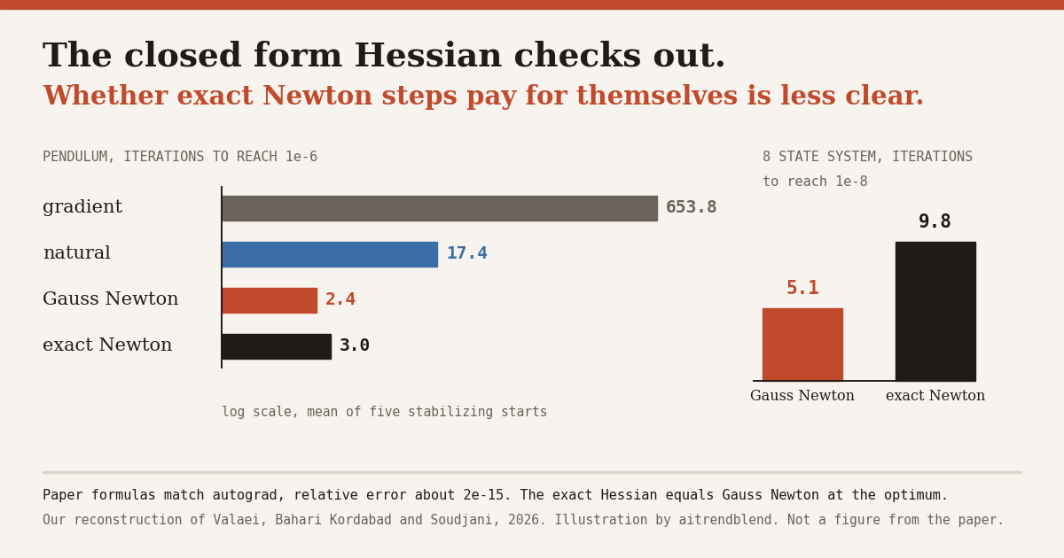
- In our toy runs exact Newton did not beat Gauss Newton. On a pendulum they needed 3.0 and 2.4 iterations, and on a random 8 state system 9.8 and 5.1, against 654 and 17 for gradient and natural gradient steps on the pendulum.
- The setting assumes a known model, so a Riccati solve already gives the optimal gain, which the authors use as their reference. The paper releases no code, and its data are available on request.
Why curvature matters for a learned controller
The linear quadratic regulator, or LQR, is the simplest serious problem in control. The system is linear, so the next state is a matrix times the current state plus a matrix times the input plus random noise. The cost adds up a quadratic penalty on how far the state strays and a quadratic penalty on how hard the input works. The best controller is a plain feedback law, the input equals minus a gain matrix times the state, and a textbook recipe called the Riccati equation delivers that gain when the matrices are known.
Reinforcement learning researchers love LQR for an odd reason. It is the one problem where the policy gradient, the value function and the cost surface all have exact formulas, so a new algorithm can be tested against the truth. Earlier work by Fazel and colleagues showed that plain policy gradient steps converge to the optimal gain even though the cost surface is not convex. The catch is speed. First order steps converge at a linear rate, and on a badly scaled problem they zigzag across a narrow valley.
Curvature fixes the zigzag. A Newton step looks at the second derivative of the cost, the Hessian, and aims straight at the bottom of the valley. In reinforcement learning this idea shows up as natural gradients and trust regions, which use cheaper stand ins for the Hessian. The exact Hessian is rarely tried, because it has two parts. One part is the curvature of the action value function, which is manageable. The other part measures how the policy changes the distribution of states the system visits, and that part needs derivatives of the transition kernel.
The paper’s bet is that LQR is simple enough for both parts to come out in closed form. If so, an exact Newton method for a control policy becomes a few lines of matrix algebra. Our earlier coverage of deep reinforcement learning controllers, such as Meta TD3 for vibration control, lived at the other end of the scale, with neural policies and no closed forms at all. This paper sits where the mathematics is exact and the system is small.
What the paper derives
The setting
The system is the discrete time linear one described above, driven by independent noise with zero mean and covariance \(\Sigma_w\). The cost is discounted by a factor \(\gamma\) below one, which is needed for a reason the authors state in a remark. With additive noise and no discounting the long run cost diverges, so \(\gamma\) must be below one for the value function to exist. The policy is a linear feedback with gain \(K\), and the learner tunes the stacked entries \(\theta = \mathrm{vec}(K)\). The gain must be gamma stabilizing, which means the closed loop matrix \(A_\theta = A – BK\) satisfies \(\rho(\sqrt{\gamma}\,A_\theta) < 1\). The performance function \(J(\theta)\) is the expected value of the value function over the starting state.
Everything else follows from two matrices. The first is the value matrix, which solves a discounted Lyapunov equation. The second is the discounted state covariance, which solves a dual one.
The gradient and the two parts of the Hessian
With those two matrices the policy gradient has a short closed form. It is a gain sized residual multiplied by the state covariance.
The general decomposition that the paper builds on comes from earlier work by Kordabad and coauthors in 2022. It splits the Hessian into a curvature term and a distribution term.
For LQR the first term collapses to a Kronecker product. The policy is linear, so its own second derivative is zero, and what remains is the curvature of the action value function scaled by the state covariance. The paper shows this is the classical Gauss Newton matrix for LQR.
The second term is the new result. It captures how the visited states shift as the gain changes, and it needs the derivative of the value matrix with respect to the gain. That derivative has its own closed form, obtained by differentiating the Lyapunov equation and vectorizing it.
One detail in those formulas shapes everything that follows. The residual \(S_\theta\) is the same gain sized quantity that sits inside the gradient, and it is zero at the optimal gain. It appears inside the Jacobian, so the transition term \(\Lambda\) is zero at the optimum. The paper notes this as a known property, that the cheap curvature term is exact there. It also means the extra work of the exact Hessian pays off only away from the optimum.
| Update rule | Preconditioner | What one step needs | Convergence the paper cites |
|---|---|---|---|
| Policy gradient | The identity | The gradient, which needs the value matrix and the state covariance | Linear, with global guarantees from earlier work |
| Natural gradient | The Fisher matrix, proportional to the state covariance Kronecker identity | The same two matrices | Linear, not equal to Gauss Newton |
| Gauss Newton | The matrix \(H(\theta)\) | The same two matrices plus a Kronecker product | Local, strong near the optimum |
| Exact Newton | \(H(\theta) + \gamma\Lambda(\theta)\) | Also the Jacobian of the value matrix, a solve of order \(n^2\) | Local, quadratic near the optimum |
Assembled from Section 2 and Section 3 of the paper. The paper states that first order methods have global convergence guarantees while Newton and Gauss Newton methods primarily have local ones.
The assumption behind the exact term
The exact Hessian needs one more condition, because differentiating the state distribution means differentiating the noise density. Assumption 2 asks that the noise has either bounded support with a piecewise smooth boundary, or a smooth density whose tails decay fast enough that boundary terms vanish. Gaussian and Laplace noise qualify, and so do truncated distributions. Heavy tailed noise does not, and if the condition fails the Hessian gains an extra boundary term that depends on the particular distribution. That is a modest restriction for engineering systems, and the authors spell it out with a full proof in the appendices.
The price tag
The matrix \(T_\theta\) has order \(n^2\), where \(n\) is the number of states, and solving with it dominates the cost. The authors state a cost of order \(n^6\) per iteration for the exact method and describe it as practical for moderate dimensions. For a 48 state benchmark that is a 2304 by 2304 system at every step. The Hessian itself is only \(mn\) by \(mn\) for \(m\) inputs, which is small. The size of the system matrices, not the number of policy parameters, is what makes the method expensive.
What the experiments show
The paper is short, eight pages with three experiments, and the experiments are meant to confirm the algebra and illustrate the speed gain. Two of them are figures with no printed numbers, and the third gives a single line of wall clock times.
| Experiment | States | Setup in the paper | What it is used for |
|---|---|---|---|
| Scalar LQR | 1 | Analytic formulas for every term, the earlier 2022 result recovered with a = b = 1 and Q = R = 0.5 | Confirms that the new expressions reproduce the exact Hessian |
| Inverted pendulum | 2 | Discount 0.9, anisotropic state penalty with eigenvalues 100000 and 0.0001 rotated by 40 degrees, input penalty 0.1, backtracking line search | Figure 1, Newton follows the valley while first order steps zigzag |
| Seismic shear building | 48 | 24 interstory displacements and 24 velocities, sample time 0.01 seconds, 10 stabilizing starting gains, fixed step sizes 0.5 for Gauss Newton and 1 for Newton | Figure 2 and the wall clock times |
From Section 4 of the paper. The pendulum discretization step and the number of inputs of the building model are not stated in the text we read.
The pendulum and the building
On the pendulum the authors plot the cost surface for two of the gain entries and overlay the paths of first order and Newton steps. The first order path wobbles across the valley and Newton goes straight to the bottom in a few steps. That is what the textbook predicts for a valley stretched by a factor of a billion, which the eigenvalues 100000 and 0.0001 create, and it makes a clear picture.
The building benchmark gives the only quantitative comparison. Figure 2 plots the distance between the current gain and the optimal gain, averaged over 10 random stabilizing starts, for natural gradient, a method the figure labels quasi Newton, which is the Gauss Newton update, and exact Newton. Reading the plot by eye, since it prints no values, exact Newton flattens out after about 8 iterations at a very low error. Gauss Newton keeps descending until about iteration 22 and then levels off at a higher error, well above Newton on the log axis. Natural gradient is still falling at iteration 30 and ends near the top of the plot.
| Method | Mean wall clock over 10 trials | Relative to natural gradient, our arithmetic |
|---|---|---|
| Natural gradient | 0.0856 seconds | 1 times |
| Gauss Newton | 0.3563 seconds | 4.2 times |
| Exact Newton | 5.7520 seconds | 67 times |
From the text of Section 4.3. Exact Newton solves linear systems of dimension 2304 by 2304 in this 48 state example. The paper does not say how many iterations each method ran or what accuracy the times correspond to.
The authors draw a modest conclusion. Newton type methods converge much faster than first order ones, Gauss Newton is a favorable trade between speed and cost, and exact Newton pays a large per iteration price for fewer iterations. They then add that such methods may be especially useful when data are limited but computation is available, because they converge faster in terms of sample efficiency.
“Such methods can be particularly useful in settings where data is limited but computational resources are available, as they achieve faster convergence in terms of sample efficiency.”Valaei and colleagues, Section 4.3
That last claim looks ahead of the evidence. No samples are drawn anywhere in the paper. The system matrices are known, the formulas are exact, and the experiments count iterations and seconds. Sample efficiency belongs to a later model free version that the authors describe as future work.
We checked the algebra
The most useful thing we could add was an independent test of the formulas, because a closed form for a Hessian is easy to get wrong by a transpose or a factor of two. Our PyTorch file builds the value matrix and the state covariance by solving the two linear systems, forms the cost \(J(\theta)\) as the trace of the value matrix against the covariance, and then asks automatic differentiation for the true gradient and Hessian. It compares those with Equations 16, 19 and 21 to 23 on a random system with 3 states and 2 inputs and a discount of 0.9.
| Quantity checked | Result |
|---|---|
| Gradient from Eq. 16 against autograd | relative error \(1.2\times10^{-15}\) |
| Exact Hessian \(H+\gamma\Lambda\) against autograd | relative error \(1.9\times10^{-15}\) |
| Gauss Newton matrix \(H\) alone against autograd | relative error 0.875 |
| \(\lVert\Lambda\rVert\) over \(\lVert\nabla^2 J\rVert\) at the Riccati optimum | \(6.9\times10^{-16}\) |
| Gradient norm at the Riccati optimum | \(2.3\times10^{-14}\) |
Our own reconstruction in float64, not a result from the paper. The Riccati optimum comes from value iteration on the discounted Riccati equation.
The formulas hold. Both the gradient and the exact Hessian agree with automatic differentiation to rounding error, and the Gauss Newton matrix alone is off by 87.5 percent away from the optimum, which shows that the transition term is not a small correction. At the optimum the transition term is zero to machine precision, as the structure of the Jacobian predicts. This is a real endorsement of the paper’s mathematics, and it is the part of the work that seems solid.
Does exact Newton beat Gauss Newton
With correct formulas in hand we ran the update rules. On the pendulum, built from the paper’s numbers with an Euler step of 0.05 seconds that we chose, we started from five stabilizing gains near the optimum and counted iterations to bring the distance to the optimal gain below \(10^{-6}\). All four methods used a backtracking line search.
| Update rule | Pendulum, 2 states, iterations to \(10^{-6}\) | Random 8 states and 3 inputs, iterations to \(10^{-8}\) |
|---|---|---|
| Policy gradient | 653.8 | not run |
| Natural gradient | 17.4 | not run |
| Gauss Newton | 2.4 | 5.1 |
| Exact Newton | 3.0 | 9.8 |
Our own reconstruction. Mean iterations over 5 starts on the pendulum and over 10 starts on the random system. The starts lie near the edge of the stabilizing set, and our code adds damping when a Hessian is not positive definite.
Curvature helps enormously over plain gradient steps, 654 iterations against 3 or fewer. The comparison between the two curvature methods is where our result differs from the paper’s figure. With a line search that starts at the full step, Gauss Newton took 2.4 iterations on the pendulum against 3.0 for exact Newton, and on the random 8 state system it took 5.1 against 9.8. Exact Newton was slower in iterations on both. The paper’s Figure 2 shows Gauss Newton lagging, but it uses a fixed step of 0.5 for Gauss Newton and 1 for Newton, which would be expected to slow Gauss Newton to a linear rate.
The reason is visible in the transition term. At our starting gains, the term \(\gamma\Lambda\) carried on average 79 percent of the Hessian’s norm, and at the worst start essentially all of it. The exact Hessian far from the optimum can be indefinite, so Newton needs damping, and the extra term pulls the direction away from what works well in the final approach. Near the optimum the two matrices coincide. This is our reading of a small experiment, not a general law, and the paper’s building is a very different system from ours. It does suggest that the exact term helps least where the paper’s local guarantees apply and misleads most where they do not.
The cost of the exact term
We also timed one exact Hessian assembly for single input systems of growing size on our CPU. The times are machine dependent and vary from run to run, so treat them as orders of magnitude.
| States n | Order of the system, n squared | Seconds for one exact Hessian |
|---|---|---|
| 8 | 64 | 0.0012 |
| 16 | 256 | 0.0052 |
| 24 | 576 | 0.0761 |
| 32 | 1024 | 0.1693 |
| 48 | 2304 | 1.2307 |
Our own reconstruction, timings from one run. A fit over the last three sizes gave a growth exponent of about 4 here and 4.7 in an earlier run, below the worst case of 6 that a dense solve of order n squared implies.
At 48 states one assembly took about 1.2 seconds on our machine. The paper reports 5.75 seconds for a whole Newton run, which is the same order as a handful of such assemblies, though the paper does not give an iteration count to check against. The practical limit sits at a few hundred states, where a dense system of order \(n^2\) no longer fits in memory.
Where the claims stretch
The baseline in the quantitative figure
The abstract says the second order approach converges faster than the standard first order policy gradient baseline. In the building benchmark, the only first order method is natural gradient, a preconditioned method that the authors themselves say is not equivalent to Gauss Newton. Plain policy gradient appears only in the pendulum picture, which has no numbers. Natural gradient is usually a stronger baseline than plain gradient, so the quantitative claim may be conservative, but the abstract’s wording is looser than the evidence.
Wall clock without a stopping rule
Natural gradient is fastest in wall clock time at 0.0856 seconds, and at the end of the plot it has not converged. The paper does not say whether the times cover a fixed 30 iterations or a run to a tolerance, so the times cannot be turned into time to a given accuracy. Without that, the 67 times figure says what one run costs and not what a good answer costs. The conclusion that exact Newton buys speed per iteration at a high price per iteration is fair, and the net benefit in time is unknown.
A known model and a known answer
Every experiment assumes the matrices \(A\), \(B\), \(Q\) and \(R\) are known. In that setting the optimal gain is one Riccati solve away, and the authors use the Riccati solution as the target for their error measure. The pendulum run starts from a gain computed with a standard LQR routine. A policy gradient method for a known LQR is therefore a test bed and not a competitor to the direct solution. Its value is as a building block for the model free settings that the conclusion lists as future work, where \(\Sigma_\theta\) and \(P_\theta\) must be estimated from trajectories.
The paper delivers a theorem and a derivation, with experiments that confirm it and illustrate the speed. It does not deliver a ready algorithm for learning controllers from data. Both the closed forms and our check of them are exact in the known model setting. Whether the transition term can be estimated reliably from samples is the open question, and the paper says so.
Step sizes and safeguards
The paper notes that Newton and Gauss Newton methods have local guarantees and usually need line search or trust regions for global behavior. The building benchmark uses fixed step sizes taken from earlier convergence results, 0.5 for Gauss Newton and 1 for Newton, and the pendulum uses backtracking. The text does not say how a non positive definite exact Hessian is handled, which our own run needed to address with damping. Different step policies would change the relative ordering of the curves, as our experiment shows.
Scale and variety
The largest test has 48 states, a single dynamics family and Gaussian noise. The number of inputs of the building model is not stated in the text we read. The starting gains are drawn by perturbing the optimal gain with Gaussian noise of 0.5 and keeping the stabilizing ones, so the starts are tied to the answer and not drawn independently of it. Nothing tests heavy tailed noise, where Assumption 2 fails, or an inexact model, and the paper says robustness under model uncertainty is future work.
Reproducibility
The paper lists no code repository, and the data availability statement is short.
“Data will be made available on request.”Valaei and colleagues, Data availability statement
The building model is referenced to an earlier work by Antoulas and coauthors, and the pendulum discretization is not given. A reader can rebuild the formulas from the paper, as we did, but not the exact experiments.
Limitations the paper states, and the ones it leaves open
The authors state their boundaries clearly. The derivation is for a known model and the exact term costs order \(n^6\) per iteration, so it suits moderate dimensions. The exact Hessian needs a tail condition on the noise. Newton type methods give local guarantees only. The conclusion lists model free curvature estimation with finite sample guarantees, actor critic and off policy variants, and robustness under model uncertainty as future work, and says that sample efficient approximations of the transition dependent Hessian term are an open challenge.
The open points are the ones above. Iteration counts and accuracy targets for each method would turn the wall clock times into a fair comparison. A plain first order baseline in the building benchmark would match the abstract’s wording. A comparison with a direct Riccati or Hewer style policy iteration would show where gradient methods stand when the model is known. And a test on larger systems and on non Gaussian noise would show whether the exact term earns its cost. None of these undermines the algebra, which our check supports, and all of them affect how much weight to put on the experimental story.
A PyTorch version of the formulas
The paper shares no code, so everything in this section is our own independent reconstruction from its equations. The file is written for checking and playing, not for speed. It builds a discounted LQR, solves for the value matrix and the state covariance with dense linear systems, and implements the closed forms from the paper next to automatic differentiation of the cost, so any disagreement shows up immediately.
Four update rules sit on top, a plain gradient step, a natural gradient step with the Fisher matrix proportional to the state covariance, a Gauss Newton step and an exact Newton step. All four use a backtracking line search that also rejects gains outside the stabilizing set. The optimal gain comes from value iteration on the discounted Riccati equation, so the error measure does not depend on the code under test.
Several choices are ours, and the code marks each as a design choice. The pendulum uses an Euler step of 0.05 seconds, since the paper does not give one. Newton and Gauss Newton add diagonal damping until the matrix is positive definite, which the paper does not describe. The random test systems and their starting gains are invented, and the starts are kept close to the optimum because the stabilizing set is thin. Vectorization stacks columns, matching the paper’s definition, and a commutation matrix is built explicitly so that the transpose identity used in the Jacobian holds.
"""
Second order policy gradient for the discounted stochastic LQR, a small
reference reconstruction.

Written by aitrendblend from the published description in Valaei, Bahari
Kordabad and Soudjani, Engineering Applications of Artificial Intelligence 184
(2026) 116312. It is NOT the authors' code. The paper lists no code and says
data are available on request.

What this file does
  1. Builds the closed forms of the paper for J(K), its gradient (Eq 16), the
     Gauss Newton matrix H (Eq 19) and the transition term Lambda (Eq 21 to 23).
  2. Checks all of them against automatic differentiation of J.
  3. Runs first order, natural, Gauss Newton and exact Newton updates on a
     rotated, badly conditioned pendulum like system.
  4. Times one exact Hessian assembly as the state dimension grows.

Design choices the paper does not fix are marked DESIGN.
Convention. vec stacks columns, theta = vec(K), K is m by n, a = -K s.
"""
import time
import torch

torch.set_default_dtype(torch.float64)
torch.manual_seed(0)


# ----------------------------------------------------------------------------
# Linear algebra helpers
# ----------------------------------------------------------------------------
def vec(X):
    return X.T.reshape(-1)


def unvec(v, rows, cols):
    return v.reshape(cols, rows).T


def commutation(m, n):
    """K_mn with vec(X^T) = K_mn vec(X) for X of shape m by n."""
    k = torch.zeros(m * n, m * n)
    for i in range(m):
        for j in range(n):
            k[i * n + j, j * m + i] = 1.0
    return k


def kron(a, b):
    a, b = a.contiguous(), b.contiguous()
    return (a[:, None, :, None] * b[None, :, None, :]).reshape(a.shape[0] * b.shape[0], a.shape[1] * b.shape[1])


# ----------------------------------------------------------------------------
# Discounted LQR quantities
# ----------------------------------------------------------------------------
class LQR:
    def __init__(self, A, B, Q, R, Sw, S0, gamma):
        self.A, self.B, self.Q, self.R = A, B, Q, R
        self.Sw, self.S0, self.gamma = Sw, S0, gamma
        self.n, self.m = A.shape[0], B.shape[1]

    def closed_loop(self, K):
        return self.A - self.B @ K

    def is_stabilizing(self, K):
        Acl = self.closed_loop(K)
        return torch.linalg.eigvals(Acl).abs().max().item() * self.gamma ** 0.5 < 1.0

    def P(self, K):
        """Eq 8, P = Q + K'RK + gamma Acl' P Acl, solved as a linear system."""
        n = self.n
        Acl = self.closed_loop(K)
        T = torch.eye(n * n) - self.gamma * kron(Acl.T, Acl.T)
        rhs = vec(self.Q + K.T @ self.R @ K)
        return unvec(torch.linalg.solve(T, rhs), n, n)

    def Sigma(self, K):
        """Eq 18, Sigma - gamma Acl Sigma Acl' = S0 + gamma/(1-gamma) Sw."""
        n = self.n
        Acl = self.closed_loop(K)
        T = torch.eye(n * n) - self.gamma * kron(Acl, Acl)
        rhs = vec(self.S0 + self.gamma / (1 - self.gamma) * self.Sw)
        return unvec(torch.linalg.solve(T, rhs), n, n)

    def J(self, K):
        """J = E[V(s0)] = tr(P S0) + gamma/(1-gamma) tr(P Sw)."""
        P = self.P(K)
        return torch.trace(P @ (self.S0 + self.gamma / (1 - self.gamma) * self.Sw))

    # -- closed forms from the paper ------------------------------------------------
    def grad(self, K):
        """Eq 16, 2 (R K - gamma B' P Acl) Sigma, returned as vec."""
        P, S = self.P(K), self.Sigma(K)
        E = self.R @ K - self.gamma * self.B.T @ P @ self.closed_loop(K)
        return vec(2 * E @ S)

    def gauss_newton(self, K):
        """Eq 19, H = 2 Sigma kron (R + gamma B' P B)."""
        P, S = self.P(K), self.Sigma(K)
        return 2 * kron(S, self.R + self.gamma * self.B.T @ P @ self.B)

    def jacobian_P(self, K, P=None):
        """Eq 22 and 23, d vec(P) / d theta."""
        n, m = self.n, self.m
        P = self.P(K) if P is None else P
        Acl = self.closed_loop(K)
        S = self.R @ K - self.gamma * self.B.T @ P @ Acl
        T = torch.eye(n * n) - self.gamma * kron(Acl.T, Acl.T)
        inner = kron(S.T, torch.eye(n)) @ commutation(m, n) + kron(torch.eye(n), S.T)
        return torch.linalg.solve(T, inner)

    def Lambda(self, K):
        """Eq 21, the transition dependent part of the Hessian."""
        P, Sg = self.P(K), self.Sigma(K)
        Acl = self.closed_loop(K)
        D = self.jacobian_P(K, P)
        left = kron(Sg @ Acl.T, self.B.T) @ D
        return -2 * (left + left.T)

    def exact_hessian(self, K):
        return self.gauss_newton(K) + self.gamma * self.Lambda(K)


def discounted_riccati_gain(sys, iters=5000):
    """Optimal gain by value iteration on the discounted Riccati equation."""
    P = sys.Q.clone()
    g = sys.gamma
    for _ in range(iters):
        G = torch.linalg.solve(sys.R + g * sys.B.T @ P @ sys.B, g * sys.B.T @ P @ sys.A)
        Pn = sys.Q + g * sys.A.T @ P @ sys.A - g * sys.A.T @ P @ sys.B @ G
        if (Pn - P).abs().max() < 1e-14 * Pn.abs().max():
            P = Pn
            break
        P = Pn
    return torch.linalg.solve(sys.R + g * sys.B.T @ P @ sys.B, g * sys.B.T @ P @ sys.A)


# ----------------------------------------------------------------------------
# Update rules
# ----------------------------------------------------------------------------
def backtrack(sys, K, d, g, alpha0=1.0, c=1e-4, shrink=0.5, tries=40):
    J0 = sys.J(K).item()
    slope = float(g @ vec(d))
    a = alpha0
    for _ in range(tries):
        Kn = K + a * d
        if sys.is_stabilizing(Kn):
            Jn = sys.J(Kn).item()
            if Jn <= J0 + c * a * slope:
                return Kn
        a *= shrink
    return K


def step_gd(sys, K):
    g = sys.grad(K)
    return backtrack(sys, K, unvec(-g, sys.m, sys.n), g, alpha0=1e-2)


def step_natural(sys, K):
    """Natural gradient with Fisher proportional to Sigma kron I, so the
    preconditioned direction drops Sigma from Eq 16."""
    P = sys.P(K)
    E = sys.R @ K - sys.gamma * sys.B.T @ P @ sys.closed_loop(K)
    return backtrack(sys, K, -2 * E, sys.grad(K), alpha0=0.5)


def spd_solve(Hm, g, floor=1e-10):
    """DESIGN, add damping until the Hessian is positive definite."""
    delta = 0.0
    eye = torch.eye(Hm.shape[0])
    for _ in range(60):
        try:
            L = torch.linalg.cholesky(Hm + delta * eye)
            return torch.cholesky_solve(g.unsqueeze(1), L).squeeze(1)
        except RuntimeError:
            delta = max(2 * delta, floor * Hm.abs().max().item())
    return g


def step_gauss_newton(sys, K):
    g = sys.grad(K)
    d = -spd_solve(sys.gauss_newton(K), g)
    return backtrack(sys, K, unvec(d, sys.m, sys.n), g, alpha0=1.0)


def step_newton(sys, K):
    g = sys.grad(K)
    d = -spd_solve(sys.exact_hessian(K), g)
    return backtrack(sys, K, unvec(d, sys.m, sys.n), g, alpha0=1.0)


def run(sys, K0, step, Kstar, tol=1e-6, max_iter=3000):
    K, t0, hist = K0.clone(), time.time(), []
    for it in range(max_iter):
        err = (K - Kstar).norm().item()
        hist.append(err)
        if err < tol:
            return it, time.time() - t0, err, hist
        K = step(sys, K)
    return max_iter, time.time() - t0, (K - Kstar).norm().item(), hist


# ----------------------------------------------------------------------------
# Test systems
# ----------------------------------------------------------------------------
def pendulum(gamma=0.9, ts=0.05):
    """Rotated, badly conditioned pendulum. Euler discretization with Ts = 0.05
    is DESIGN, the paper only says discretized upright linearization."""
    g, l, mass = 9.81, 1.0, 1.0
    Ac = torch.tensor([[0.0, 1.0], [g / l, 0.0]])
    Bc = torch.tensor([[0.0], [1.0 / (mass * l * l)]])
    A, B = torch.eye(2) + ts * Ac, ts * Bc
    c, s = torch.cos(torch.tensor(40 * 3.14159265 / 180)), torch.sin(torch.tensor(40 * 3.14159265 / 180))
    C = torch.stack([torch.stack([c, -s]), torch.stack([s, c])])
    Q = C @ torch.diag(torch.tensor([1e5, 1e-4])) @ C.T
    return LQR(A, B, Q, torch.tensor([[0.1]]), torch.eye(2), 0.1 * torch.eye(2), gamma)


def random_system(n, m, gamma=0.9, seed=1):
    gen = torch.Generator().manual_seed(seed)
    A = torch.randn(n, n, generator=gen) * 0.5
    B = torch.randn(n, m, generator=gen)
    M = torch.randn(n, n, generator=gen)
    Q = M @ M.T / n + 0.1 * torch.eye(n)
    N = torch.randn(m, m, generator=gen)
    R = N @ N.T + 0.5 * torch.eye(m)
    return LQR(A, B, Q, R, 0.2 * torch.eye(n), 0.5 * torch.eye(n), gamma)


# ----------------------------------------------------------------------------
# Smoke test
# ----------------------------------------------------------------------------
if __name__ == "__main__":
    # 1. closed forms against automatic differentiation
    sys3 = random_system(3, 2)
    K = torch.randn(2, 3) * 0.3
    while not sys3.is_stabilizing(K):
        K = K * 0.5
    th = vec(K)
    f = lambda v: sys3.J(unvec(v, 2, 3))
    g_auto = torch.autograd.functional.jacobian(f, th)
    H_auto = torch.autograd.functional.hessian(f, th)
    g_cf, H_gn, Lam = sys3.grad(K), sys3.gauss_newton(K), sys3.Lambda(K)
    H_ex = H_gn + sys3.gamma * Lam
    rel = lambda a, b: ((a - b).norm() / b.norm()).item()
    print("Closed forms against autograd on a random 3 state, 2 input system")
    print(f"  gradient, Eq 16               relative error {rel(g_cf, g_auto):.2e}")
    print(f"  exact Hessian, H + gamma Lam  relative error {rel(H_ex, H_auto):.2e}")
    print(f"  Gauss Newton H alone          relative error {rel(H_gn, H_auto):.2e}")
    Kst = discounted_riccati_gain(sys3)
    Lam_star = sys3.Lambda(Kst)
    print(f"  at the optimum, |Lambda| / |Hessian| = {(Lam_star.norm() / sys3.exact_hessian(Kst).norm()).item():.2e}")
    print(f"  at the optimum, |gradient| = {sys3.grad(Kst).norm().item():.2e}")
    assert rel(g_cf, g_auto) < 1e-6 and rel(H_ex, H_auto) < 1e-6

    # 2. update rules on the pendulum
    sysp = pendulum()
    Kstar = discounted_riccati_gain(sysp)
    gen = torch.Generator().manual_seed(3)
    results = {k: [] for k in ("gradient", "natural", "Gauss Newton", "Newton")}
    steps = {"gradient": step_gd, "natural": step_natural,
             "Gauss Newton": step_gauss_newton, "Newton": step_newton}
    for trial in range(5):
        while True:
            K0 = Kstar + 0.5 * torch.randn(1, 2, generator=gen)
            if sysp.is_stabilizing(K0):
                break
        for name, st in steps.items():
            it, secs, err, _ = run(sysp, K0, st, Kstar, tol=1e-6, max_iter=3000)
            results[name].append((it, secs, err))
    print("\nPendulum, gamma 0.9, five stabilizing starts, tolerance 1e-6 on |K - K*|")
    for name, rows in results.items():
        its = torch.tensor([r[0] for r in rows], dtype=torch.float64)
        sec = torch.tensor([r[1] for r in rows])
        errs = torch.tensor([r[2] for r in rows])
        print(f"  {name:13s} iterations {its.mean():7.1f}  seconds {sec.mean():7.4f}  final error {errs.max():.1e}")

    # 2b. Gauss Newton against exact Newton on a larger random system
    sysb = random_system(8, 3, seed=11)
    Kb = discounted_riccati_gain(sysb)
    gen2 = torch.Generator().manual_seed(5)
    print("\nRandom 8 state, 3 input system, ten stabilizing starts, tolerance 1e-8")
    rows = {"Gauss Newton": [], "Newton": []}
    shares = []
    for trial in range(10):
        for _ in range(500):
            K0 = Kb + 0.12 * torch.randn(3, 8, generator=gen2)
            if sysb.is_stabilizing(K0):
                break
        shares.append((sysb.gamma * sysb.Lambda(K0).norm() / sysb.exact_hessian(K0).norm()).item())
        for name, st in (("Gauss Newton", step_gauss_newton), ("Newton", step_newton)):
            it, secs, err, _ = run(sysb, K0, st, Kb, tol=1e-8, max_iter=200)
            rows[name].append((it, secs, err))
    for name, r in rows.items():
        print(f"  {name:13s} iterations {sum(x[0] for x in r) / len(r):5.1f}  seconds {sum(x[1] for x in r) / len(r):7.4f}  worst final error {max(x[2] for x in r):.1e}")
    print(f"  share of the Hessian carried by gamma Lambda at the start, mean {sum(shares) / len(shares):.2f}, max {max(shares):.2f}")

    # 3. cost of one exact Hessian as n grows
    print("\nTime for one exact Hessian assembly, single input system")
    ns, ts = [8, 16, 24, 32, 48], []
    for n in ns:
        s = random_system(n, 1, seed=n)
        Kn = discounted_riccati_gain(s)
        s.exact_hessian(Kn)
        t0 = time.time()
        s.exact_hessian(Kn)
        ts.append(time.time() - t0)
        print(f"  n = {n:2d}   matrix of order {n * n:3d}   {ts[-1]:.4f} s")
    import numpy as np
    slope = np.polyfit(np.log(ns[-3:]), np.log(ts[-3:]), 1)[0]
    print(f"  growth exponent over the last three sizes {slope:.2f}")
    assert results["Newton"][0][2] < 1e-5
    print("\nsmoke test passed")
The smoke test runs three things. It compares the closed forms with automatic differentiation on a random 3 state system, runs the four updates on the pendulum and the two curvature updates on a random 8 state system, and times one exact Hessian assembly for growing sizes.
The first block is the one that matters. Both the gradient and the exact Hessian agree with automatic differentiation to about \(10^{-15}\), the Gauss Newton matrix alone does not, and the transition term vanishes at the optimum together with the gradient. We went in expecting a transposition error somewhere, since the Kronecker algebra is unforgiving, and found none. The authors’ formulas and our reading of them are consistent.
The second block shows what curvature buys on a badly scaled problem. Plain gradient steps needed 654 iterations on average and about five seconds, natural gradient needed 17, and both curvature methods needed 3 or fewer. The third block is the surprise. Starting near the edge of the stabilizing set of a random 8 state system, exact Newton needed 9.8 iterations against 5.1 for Gauss Newton and cost four times as much time. Whether that holds for the paper’s building we cannot say, but it is a reminder that the exact Hessian is a tool whose value depends on where the iteration starts.
The exact Hessian and the Gauss Newton matrix coincide at the optimum, and the difference between them grows with the policy residual. If you reuse these formulas, measure how large the transition term is along your own path before paying for it, and keep a damping rule ready for the stretches where the exact matrix is not positive definite.
What this adds up to
The paper’s contribution is a clean piece of mathematics. For discounted stochastic LQR, the exact Hessian of the cost with respect to a feedback gain has a closed form. It splits into a Gauss Newton term, built from the action value curvature and the state covariance, and a transition term that comes from the value matrix and its Jacobian. The authors prove the decomposition with careful treatment of the noise density, state the condition under which it holds, and show that it reduces to an earlier scalar result. Our independent check agrees to rounding error, which is more than most theory papers can say about their formulas.
The experimental story is thinner and should be read as illustration. A pendulum picture shows Newton steps cutting across a stretched valley, and a 48 state building shows second order updates converging in far fewer iterations than natural gradient. The price is stated openly, 0.3563 seconds for Gauss Newton and 5.7520 seconds for exact Newton against 0.0856 for natural gradient, and the paper does not give iteration counts or accuracy targets that would turn those times into a comparison at equal quality. The claim about sample efficiency, which appears at the end of the building section, is untested because no samples are drawn.
Our own runs add a caution. Curvature helps enormously over plain gradient steps, and exact Newton came close to Gauss Newton on a pendulum, but it needed about twice as many iterations on a random 8 state system. The cause is plausible and visible in the numbers. The transition term is zero at the optimum and large away from it, and far from the optimum the exact Hessian can lose positive definiteness. This is a small experiment on invented systems, and it should be read as a prompt for more testing and not as a verdict on the paper.
The setting also deserves a plain statement. With a known model, the optimal gain is one Riccati solve away, and the authors use that very solution as their reference. The value of the work is as a foundation for the situation where the model is unknown and \(P_\theta\) and \(\Sigma_\theta\) must be estimated from trajectories. There the exact term would have to be estimated too, and the paper names that as the open challenge. The explicit structure it provides, with every piece written in terms of quantities that the authors suggest actor critic or perturbation based methods could estimate, is the real gift to that future work.
For practitioners the guidance is concrete. If you work with small or moderate linear systems and want a curvature aware policy search, the Gauss Newton matrix of Equation 19 is cheap, exact at the optimum, and in our tests at least as good as the exact Hessian. If you want to study the geometry of policy optimization, the exact formulas are a rare gift, and they can be verified in a few dozen lines. If your noise has heavy tails, check the tail condition first. Readers who follow robot control will recognize the setting from earlier coverage of a robotized crane that exploits pendulum dynamics and of a risk aware routing policy for a warehouse robot, and more analyses on robots and autonomous systems sit in the robotic AI archive.
The road ahead, as the authors sketch it, is model free curvature estimation with finite sample guarantees and robustness to model error. Our own wish list is shorter. Release the code, report iteration counts next to wall clock times, add a plain first order baseline to the large benchmark, and test the exact term on systems where it cannot hide behind a line search. The paper ends where a good theory contribution should, with a result that is exactly right and a clear list of what remains to be learned from data.
Frequently asked questions
What does the paper actually derive?
For discounted stochastic LQR it gives closed form expressions for the policy gradient, for a Gauss Newton curvature matrix and for the exact Hessian of the cost with respect to the feedback gain. The exact Hessian is the Gauss Newton matrix plus a transition term that captures how the gain changes the distribution of visited states. The derivation needs the noise density to be smooth with fast decaying tails.
Are the formulas correct?
In our independent PyTorch check they are. On a random system with 3 states and 2 inputs, the gradient and the exact Hessian matched automatic differentiation to a relative error of about 2 parts in 10 to the 15. The Gauss Newton matrix alone was off by 87.5 percent away from the optimum, and the transition term was zero to machine precision at the optimum.
Is exact Newton faster than Gauss Newton?
Not in our tests. On a pendulum exact Newton needed 3.0 iterations against 2.4 for Gauss Newton, and on a random 8 state system 9.8 against 5.1. The paper’s 48 state figure shows exact Newton converging in fewer iterations, but it uses a fixed step of 0.5 for Gauss Newton against 1 for Newton, which favors Newton. Results depend on the system and on where the iteration starts.
How expensive is the exact Hessian?
The paper states a cost of order n to the sixth power per iteration, where n is the number of states, because it solves a system of order n squared. In its 48 state example that system is 2304 by 2304, and the mean wall clock times were 0.0856 seconds for natural gradient, 0.3563 for Gauss Newton and 5.7520 for exact Newton. The paper does not report iteration counts or the accuracy each time corresponds to.
Does this help train real controllers from data?
Not yet. Every experiment assumes the system matrices are known, in which case a Riccati solve already gives the optimal gain, and the authors use it as their reference. The paper presents the explicit formulas as a foundation for future sample based methods and lists model free curvature estimation and robustness to model error as open work. Its remark about sample efficiency is not tested, since no samples are drawn.
Can I reproduce the work?
Only partly. The paper lists no code, and its data availability statement says data will be made available on request. Our PyTorch file rebuilds the formulas from the equations, verifies them against automatic differentiation and runs the update rules on small systems in about 40 seconds on a CPU. It does not reproduce the paper’s building benchmark.
Read the paper
The article is open access under a Creative Commons license in Engineering Applications of Artificial Intelligence. The paper lists no code repository and says data are available on request, so the secondary button below leads to more analyses in the same category and not to a repository. Replace it with a repository link if one appears.
Valaei, A., Bahari Kordabad, A., and Soudjani, S. Second order policy gradient methods for the linear quadratic regulator. Engineering Applications of Artificial Intelligence 184 (2026) 116312. DOI 10.1016/j.engappai.2026.116312. Open access under a CC BY license.
This analysis is based on the published paper and an independent evaluation of its claims.