
- Uncertainty estimation
- Subclass learning
- RBF networks
- Out of distribution detection
- Feature collapse
- Single forward pass
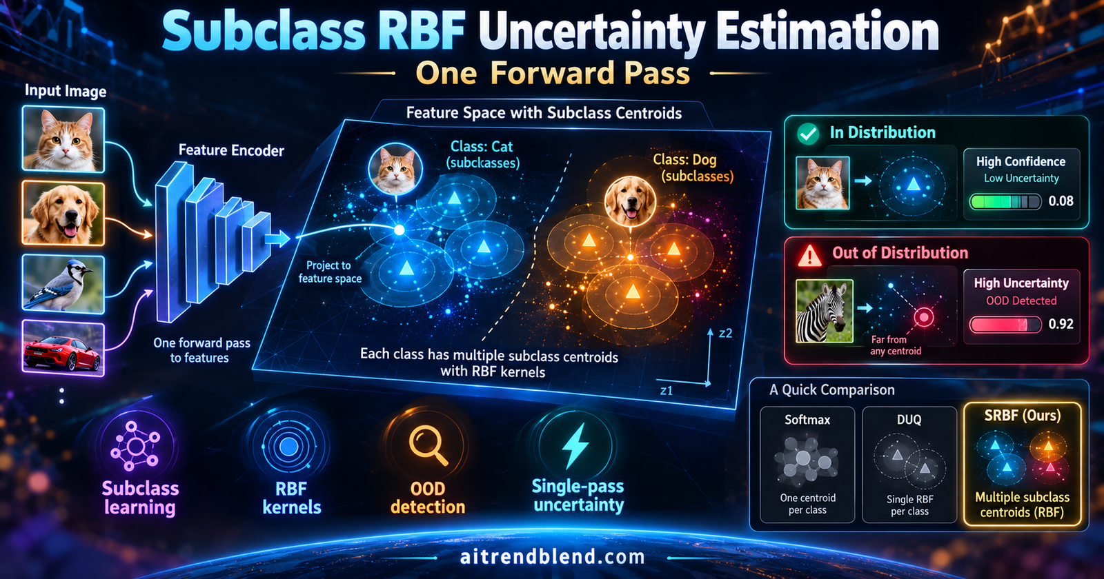
A camera above a warehouse loading door has spent months learning one job. Say whether a person is standing in the frame. It does the job well, right up to the afternoon a delivery truck backs in with a wall of mirrored panels on its side, and the classifier announces with total confidence that nobody is there.
The model never lied exactly. It was never built to say that it had no idea. Closing the gap between a confident answer and an honest one is the aim of a 2025 Neurocomputing paper from Dimitrios Spanos, Nikolaos Passalis and Anastasios Tefas at the AIIA Lab of Aristotle University of Thessaloniki, and their route is unusual. Instead of asking one network to hedge, they split every class into smaller pieces and teach the network to recognize each piece on its own.
Key points
- SRBF gives every class several centroids, one per subclass found by K means in the feature space of a pretrained autoencoder, and it reads uncertainty off a single forward pass.
- On benchmarks where the subclasses are the original dataset classes, the gains are large. FashionMNIST against MNIST reaches an AUROC of 0.9452 where DUQ reaches 0.8862, and SVHN against CIFAR-10 reaches 0.9869.
- Where the subclasses are not known, as in the Human Detection dataset, the lead nearly disappears. Against SVHN as the OOD set, SRBF scores 0.5879 and DUQ scores 0.5863.
- The ablations put the contribution of subclass learning between about 0.05 and 0.12 AUROC, while autoencoder pretraining adds less and adds it unevenly.
- Softmax, MC Dropout and ensembles score far below 0.5 on SVHN against CIFAR-10, which means their uncertainty points the wrong way and is not merely weak.
Why a confident network is a problem worth fixing
Ask a standard classifier about something it has never seen and it still has to pick a label. The softmax at the end squeezes its scores into probabilities that sum to one, so even an input unrelated to every training class comes back looking decisive. Hein, Andriushchenko and Bitterwolf explained at CVPR 2019 why ReLU networks tend to produce high confidence predictions far away from the training data, and the SRBF paper builds on that line of work. It also cites research indicating that the entropy of a softmax mostly captures aleatoric uncertainty, which is noise in the data itself, instead of the epistemic kind that tells you a model has wandered outside its experience.
The usual remedies work by asking the same question many times. Deep ensembles, introduced by Lakshminarayanan, Pritzel and Blundell in 2017, train several networks and compare their answers. MC Dropout, from Gal and Ghahramani in 2016, keeps dropout switched on at test time and samples repeatedly. Both deliver useful uncertainty. Both also multiply the cost of every prediction, which is a poor bargain for an embedded camera or a robot that has to react immediately.
That cost explains the growing interest in methods that need only one pass. The question is whether a single pass can carry enough information to tell a familiar input from a strange one.
Background and prior work
Distance as a measure of doubt
Van Amersfoort, Smith, Teh and Gal proposed one answer at ICML 2020 with DUQ, short for deterministic uncertainty quantification. The final layer becomes a Radial Basis Function layer. Each class owns a centroid, the network maps an input to a feature vector, and the kernel value between that vector and each centroid says how well the input fits that class. Uncertainty is simply how far the input sits from its nearest centroid. An input far from every centroid belongs to no known class, which is exactly the doubt a softmax cannot express.
If you follow this corner of the field, our wider coverage of uncertainty aware learning shows how distance based scoring sits next to ensembles, Bayesian methods and certification work. Our earlier analysis of adversarial robustness certification approaches the same trust question from the guarantee side.
Feature collapse, the failure DUQ had to fight
RBF training pulls training features toward their centroids. Nothing in that objective says where an unfamiliar input should land. A powerful feature extractor is free to map it right on top of familiar features, and then the distance test sees nothing wrong. Van Amersfoort and colleagues described this feature collapse in a 2021 arXiv paper, and several fixes followed. DUQ itself uses a gradient penalty, an idea that traces back to the double backpropagation of Drucker and Le Cun in 1992. Spectral normalization, from Miyato and colleagues, and residual connections, studied by Gouk and colleagues, limit how much a network can distort its feature space, and Liu and colleagues later put them to work in their distance aware models. Reversible architectures, such as the invertible networks of Jacobsen and colleagues, avoid discarding information altogether, though the authors of this paper point out that they consume more memory and are hard to train.
The gradient penalty has its own price, because it forces a second backward pass through the network. We return to that price later, since the paper makes a specific claim about it.
The assumption nobody liked to say out loud
DUQ and its relatives assume that each class forms one blob in feature space. Real classes rarely cooperate. A vehicle class in CIFAR-10 contains airplanes, automobiles, ships and trucks, which look nothing alike. One centroid has to sit somewhere in the middle of all four, and that middle ground is where plenty of unfamiliar inputs also live. Anyone who has trained a vision model on mixed categories will recognize the problem. Our computer vision hub collects more cases of benchmark classes that are really several classes in disguise.
How SRBF works
One class, several centroids
The architecture is easier to hold in your head than the paper’s notation suggests. A convolutional encoder turns an input into a feature vector. For every subclass there is a small learnable matrix that projects that vector into a lower dimensional space, a centroid in that space, and a length scale that says how forgiving the subclass is. The kernel for each subclass measures how close the projected features are to that subclass centroid.
Here \(F_\omega\) is the encoder, \(\mathbf{W}_s\) the projection for subclass \(s\), \(\mathbf{e}_s\) its centroid and \(\sigma_s\) its length scale. A class does not get its score from an average over its subclasses. It gets the best score among them, through a max pooling step, and the predicted class is the one whose best subclass fits the input most closely. Uncertainty follows directly.
This is where the design pays off in principle. A class with four visual modes no longer needs one centroid stretched across all four. Each mode gets its own, and an input that lands between modes now sits far from every centroid instead of conveniently close to the average.
The three step recipe
Training happens in three stages. First comes a plain convolutional autoencoder, trained with a mean squared reconstruction loss using Adam at a learning rate of 0.001 for 30 epochs in every experiment. The point of this stage is to keep the encoder from throwing away information that the classification task does not need. The authors connect this to mutual information maximization, citing Torkkola, and echo the variance preserving argument that Passalis and colleagues made in earlier metric learning work. Their dog breed example makes the intuition concrete. A classifier asked only to say dog has every incentive to ignore breed, and ignoring breed is exactly what makes subclasses impossible to find later.
Second, the encoder features of the training data are clustered with K means, class by class, and each cluster center becomes the starting centroid of one subclass. K means itself is the classic algorithm of Hartigan and Wong from 1979, and nothing about this step is exotic.
Third, the model trains on a binary cross entropy loss computed on the max pooled class scores, plus an L2 penalty on the encoder weights, the projection matrices and the length scales. The centroids are not trained by gradient descent at all. They follow an exponential moving average of the projected features that land on each subclass, a scheme the paper traces to the discrete representation work of van den Oord, Vinyals and colleagues and to DUQ.
Reading the equations closely
A careful reader runs into a handful of small snags, and they matter if you plan to reimplement the method. Equation 10 as printed sums the projected features of every sample in a minibatch, with no term saying which subclass a sample belongs to. A centroid built that way would be the batch mean for every subclass. The version above carries the assignment indicator, which is what the DUQ style update needs, and my implementation below assigns each sample to its best scoring subclass inside its true class.
Equation 3 writes its argument maximum over the subclass index, while Algorithm 1 takes it over the class index. The text also refers to the algorithm as Algorithm 28 when it is Algorithm 1. These look like typesetting slips and cost nothing, though they show how easy it is to misread the procedure.
The clustering step deserves more attention. Section 3.1 says clustering runs on the projected features \(F’_s(\mathbf{x})\), yet those features depend on the matrices \(\mathbf{W}_s\), which only exist once subclasses have been chosen. Algorithm 1 clusters the raw encoder output instead. The two spaces even differ in size for FashionMNIST, where the encoder emits 256 dimensions and the centroids live in 64. My code clusters the encoder features and pushes each cluster center through its own projection matrix, which is one consistent reading and the least arbitrary one I could find.
What the experiments actually show
The authors build their benchmarks from pairs of datasets, following Nalisnick and colleagues. A model trains on one dataset as a binary problem and is then asked to flag the other dataset as out of distribution. For MNIST the two classes are odd digits and even digits. For FashionMNIST they are tops and bags against trousers, dresses and footwear. For CIFAR-10 they are vehicles and animals. For Tiny ImageNet they are the first and second halves of its categories. Each result is a mean over five repetitions, and the metric is AUROC computed on the uncertainty score, where 1 means a perfect split between in domain and out of distribution data.
The headline comparison
| Setup | Softmax | MC Dropout | Ensemble of ten | DUQ | SRBF |
|---|---|---|---|---|---|
| MNIST versus FashionMNIST | 0.9064 | 0.9145 | 0.9355 | 0.8622 | 0.9380 |
| FashionMNIST versus MNIST | 0.8089 | 0.8142 | 0.8750 | 0.8862 | 0.9452 |
| CIFAR-10 versus SVHN | 0.9227 | 0.9548 | 0.8863 | 0.8300 | 0.9307 |
| SVHN versus CIFAR-10 | 0.1871 | 0.2006 | 0.3931 | 0.9100 | 0.9869 |
| Tiny ImageNet versus CIFAR-10 | 0.5028 | 0.5080 | 0.4998 | 0.5246 | 0.6118 |
| Tiny ImageNet versus SVHN | 0.6207 | 0.5910 | 0.5812 | 0.6261 | 0.6664 |
Read quickly, the table is a clean win. SRBF has the highest AUROC in five of six rows, and the margins on FashionMNIST against MNIST and on Tiny ImageNet are large. Read slowly, the picture has texture. On MNIST against FashionMNIST the SRBF score of 0.9380 comes with a standard deviation of 0.016, while the ensemble of ten sits at 0.9355 with 0.007. Those two sit well within one standard deviation of each other, so the claim that SRBF outperforms all baselines on that row is true only in the narrowest sense. On CIFAR-10 against SVHN, MC Dropout leads at 0.9548 against 0.9307, a gap the paper acknowledges while noting that MC Dropout needs many forward passes.
Using a single Gaussian component per class is insufficient for adequately separating multimodal classes. Spanos, Passalis and Tefas, Neurocomputing 651, 2025
Accuracy tells a quieter story. On CIFAR-10 SRBF reaches 95.05 percent, above DUQ at 93.14 percent and slightly below softmax at 95.47 percent. On SVHN it lands at 90.02 percent, below DUQ at 91.27 percent. On Tiny ImageNet it trails DUQ by about 0.6 points, 70.54 against 71.17, which the authors attribute to the extra variance the method keeps inside each class. None of this is alarming. It does show that the uncertainty gains are not bought with a hidden accuracy windfall.
Ask where the subclasses came from. In the headline benchmarks the paper defines the subclasses as the original dataset classes, such as the ten MNIST digits, while the comparison models are trained on the two merged classes. The paper does not say whether K means was run to recover those groups or whether the labels were used directly. Either way, SRBF starts with the right number of subclasses and a favorable layout for them.
Baselines that score below chance
The SVHN against CIFAR-10 row deserves its own look. A model that separates two datasets at random scores an AUROC of 0.5. Softmax manages 0.1871 and MC Dropout 0.2006. The ensembles reach only 0.3731, 0.3878 and 0.3931 for three, five and ten members. These are not weak detectors. They are inverted ones, assigning more confidence to the unfamiliar CIFAR-10 photographs than to the SVHN house numbers they were trained on. Flip the sign of the softmax uncertainty and the same numbers would read about 0.81.
The paper explains the effect through domain shift. A network trained on simple digit images has learned a narrow set of patterns and meets the richer natural images with the same unearned confidence. That explanation is plausible, though the paper never points out the inversion itself. For a practitioner this is the most useful line in the whole evaluation. If your detector reports an AUROC far below 0.5, the problem is not noise, it is that your uncertainty score tracks the wrong thing.
The mixture test
One experiment goes beyond dataset swaps. The authors blend an MNIST digit with an image from the opposite class, keeping a fraction p of the original, with p set to 1.0, 0.90, 0.75, 0.60 and 0.50. Confidence should fall as p falls, because the picture becomes ambiguous. Softmax and MC Dropout barely move, and by my reading of the plot they still report confidence around 94 percent at an even blend. DUQ falls to roughly 85 percent, and SRBF falls furthest, to roughly 73 percent. Those plot readings are approximate, so treat them as shape rather than measurement. The shape is still reassuring. A model that has seen a handful of tight subclasses behaves as though an even mix of two digits is a stranger to it.
Where the lead thins out
The most honest test in the paper is the one without a built in answer. The Human Detection dataset, a collection of CCTV frames from indoor and outdoor scenes, has no known subclass structure. Here SRBF has to discover its subclasses with K means, and the number of subclasses becomes a hyperparameter.
| Method | Accuracy | Tiny ImageNet | CIFAR-10 | SVHN |
|---|---|---|---|---|
| Softmax | 70.78 ± 3.14 | 0.4040 | 0.4895 | 0.5203 |
| MC Dropout | 76.52 ± 0.63 | 0.5640 | 0.6468 | 0.6191 |
| Ensemble of ten | 75.18 ± 0.25 | 0.5167 | 0.6071 | 0.6374 |
| DUQ | 73.58 ± 1.56 | 0.5623 | 0.5125 | 0.5863 |
| SRBF | 77.82 ± 0.93 | 0.6440 | 0.5487 | 0.5879 |
SRBF posts the best accuracy and the best Tiny ImageNet AUROC. On CIFAR-10 as the OOD set it trails MC Dropout by about 0.1, and against SVHN its 0.5879 is a hair above DUQ at 0.5863, with standard deviations of 0.008 and 0.002. A gap of 0.0016 is not a result.
Table 6 in the paper makes it worse. The authors chose the number of subclasses by tuning AUROC against SVHN, then reported the SVHN score at the winning setting. The scores across subclass counts are 0.5348 for three, 0.5757 for four, 0.5618 for five, 0.5786 for six, 0.5879 for seven, 0.5700 for eight, 0.5800 for nine and 0.5731 for ten. DUQ scores 0.5863. Seven of the eight settings fall below DUQ, and only the tuned one edges past it. The CIFAR-10 and Tiny ImageNet columns are genuinely held out from that tuning, which is a fair design, but the SVHN column is the best of eight draws on the same test data.
The subclass idea clearly helps when you know the subclasses. When you must discover them, the benefit in this paper is real on one OOD set, absent on another and within noise on a third. That is a more modest claim than the abstract suggests, and a more useful one for deciding whether to adopt the method.
Pretraining versus subclass learning
Two ablation tables let us separate the method’s two ingredients. Table 9 shows a single centroid model with a pretrained encoder, which isolates the effect of subclass learning. Table 8 shows the SRBF rows with and without pretraining. The checkmark column did not survive text extraction from my copy of the PDF, so I read the unbolded SRBF rows as the ones without pretraining. I read the first DUQ row of each pair the same way. That reading matches the DUQ values in Table 1 and the bolded headline scores.
| Setup | Single centroid, pretrained | SRBF, no pretraining | Full SRBF |
|---|---|---|---|
| MNIST versus FashionMNIST | 0.8821 | 0.8749 | 0.9380 |
| FashionMNIST versus MNIST | 0.8848 | 0.9132 | 0.9452 |
| CIFAR-10 versus SVHN | 0.8790 | 0.9280 | 0.9307 |
| SVHN versus CIFAR-10 | 0.9262 | 0.9507 | 0.9869 |
| Tiny ImageNet versus CIFAR-10 | 0.4919 | 0.5669 | 0.6118 |
| Tiny ImageNet versus SVHN | 0.5931 | 0.6558 | 0.6664 |
Going from a single centroid to subclasses lifts AUROC by 0.0559, 0.0604, 0.0517, 0.0607, 0.1199 and 0.0733 across the six rows. That is a steady gain. Pretraining behaves less predictably. On CIFAR-10 against SVHN the unpretrained SRBF already reaches 0.9280, and pretraining adds 0.0027, well inside the 0.016 standard deviation. On MNIST the two ingredients only work together, since each alone sits around 0.88. DUQ shows the same unevenness in Table 8. Pretraining its encoder helps on SVHN, where the score rises from 0.9100 to 0.9722, and hurts on CIFAR-10, where it drops from 0.8300 to 0.7762. In fact DUQ with a pretrained encoder beats SRBF without one on SVHN against CIFAR-10. The autoencoder is not a free gift to every method, and its value seems to depend on the dataset.
Sensitivity to regularization and batch size
The regularization sweep in Table 10 is reassuring at small values. FashionMNIST AUROC sits at 0.9472 with no L2 penalty and 0.9452 at a weight of 0.00001, and CIFAR-10 moves from 0.9244 to 0.9307 in the same step. At a weight of 0.001 the picture collapses, with AUROC at 0.8423 on FashionMNIST and 0.7288 on CIFAR-10. The batch size sweep is bumpier. FashionMNIST AUROC climbs from 0.9252 at a batch of 16 to 0.9565 at 256, then slips to 0.9214 at 1024. CIFAR-10 swings from 0.8421 with a huge standard deviation of 0.131 at a batch of 16 to 0.9349 at 32. The default of 128 is the peak for neither dataset, which suggests the reported numbers were not squeezed for every last point, and also that anyone reproducing them should budget time for tuning.
What the runtime claim does and does not show
The paper says its training overhead, at most 200 percent on MNIST and FashionMNIST and 140 percent on CIFAR-10, SVHN and Tiny ImageNet, is lower than the overhead of a gradient penalty. For the penalty it cites 380 percent, from epoch times of 103 seconds with the penalty and 27 seconds without. Those two numbers imply a slowdown of about 3.8 times, which is an overhead of roughly 281 percent, not 380. The 103 and 27 second figures also come from the DUQ paper, on that paper’s hardware, so the comparison mixes numbers measured here with numbers measured elsewhere. The baseline for the 200 and 140 percent figures is not spelled out either. The direction is plausible, since skipping double backpropagation should help, but the paper does not offer a head to head timing.
What this means in practice
The strongest practical lesson is about structure you already have. If your classes come with metadata, such as camera locations, device models, product subtypes or sensor conditions, those groupings are candidate subclasses, and the paper’s benchmark results suggest that using them can sharpen uncertainty a lot. When you have no such metadata, treat the subclass count as a hyperparameter, tune it on a validation set that includes some out of distribution data, and then test on data you did not use for tuning.
The second lesson is about measurement. Always check the direction of an out of distribution score before trusting its magnitude. The SVHN row is a reminder that an AUROC below 0.5 is a finding, not a failure to report.
The third concerns cost. A method that adds one set of small projection matrices and a handful of centroids, and needs no repeated passes at inference, is attractive for the lightweight models that dominate embedded work. Readers interested in how small models are made small can browse our knowledge distillation and compression hub, since the same deployment pressure applies. The authors themselves name autonomous vehicles and medical imaging as target fields. The paper does not validate the method in either, so any safety critical use would need its own evidence.
SRBF is best understood as a way to spend structure you already know about. Its numbers are strongest when subclasses are given, steady when pretraining and subclass learning are combined, and modest when subclasses must be discovered.
Honest limitations
Several limits come straight from the paper’s own design. The headline benchmarks use known subclasses, as discussed above, so they measure the benefit of good subclass structure and say less about discovery. The one benchmark that requires discovery shows a thin margin. The subclass count on that benchmark was tuned against one of the three reported OOD sets, which flatters that column.
The out of distribution sets are also dataset swaps, such as FashionMNIST for MNIST or SVHN for CIFAR-10. These are clean, large shifts. Real deployments meet smaller and stranger changes, a new camera angle or a slightly different lighting setup, and the paper does not test them. Each number is a mean over five runs, which is standard for this literature but thin for separating gaps of a few thousandths.
The paper says it compares against the approaches in its references 6, 8 and 38, the last being the deep deterministic uncertainty baseline of Mukhoti and colleagues. I could not find a row for that method in any table, and the text sometimes calls reference 8 DDU when reference 8 is the DUQ paper. Readers should not assume a comparison with that baseline exists. The paper also reports AUROC and accuracy but no calibration measure, so we learn nothing about whether the confidence values themselves can be taken literally.
Complete PyTorch implementation
The code below is a full reference implementation written for this article. It follows the paper’s equations, resolves the ambiguities discussed earlier in the ways described there, and ends with a smoke test on dummy data. It is an independent reading of the method and not the authors’ own repository, which is linked at the end of this page. Run the file directly to execute the smoke test.
"""
SRBF, a subclass aware RBF network for single forward pass uncertainty estimation.
Reference implementation of the method in Spanos, Passalis and Tefas,
Neurocomputing 651 (2025) 130954. Written for aitrendblend.com as an independent
reading of the paper, not the authors' official code.
"""
import math
import torch
import torch.nn as nn
import torch.nn.functional as F


# ----------------------------------------------------------------------------
# Step 1. Convolutional autoencoder used to pretrain the feature extractor
# ----------------------------------------------------------------------------
class ConvAutoencoder(nn.Module):
    """Encoder F_omega and decoder G_omega' for 28 x 28 inputs (MNIST style)."""

    def __init__(self, in_ch=1, feat_dim=64):
        super().__init__()
        self.encoder = nn.Sequential(
            nn.Conv2d(in_ch, 32, 3, stride=2, padding=1), nn.ReLU(),
            nn.Conv2d(32, 64, 3, stride=2, padding=1), nn.ReLU(),
            nn.Conv2d(64, 128, 3, stride=2, padding=1), nn.ReLU(),
            nn.AdaptiveAvgPool2d(3), nn.Flatten(),
            nn.Linear(128 * 3 * 3, feat_dim),
        )
        self.dec_fc = nn.Linear(feat_dim, 128 * 3 * 3)
        self.decoder = nn.Sequential(
            nn.ConvTranspose2d(128, 64, 3, stride=2), nn.ReLU(),                          # 3 -> 7
            nn.ConvTranspose2d(64, 32, 3, stride=2, padding=1, output_padding=1), nn.ReLU(),  # 7 -> 14
            nn.ConvTranspose2d(32, in_ch, 3, stride=2, padding=1, output_padding=1),      # 14 -> 28
            nn.Sigmoid(),
        )

    def forward(self, x):
        z = self.encoder(x)
        h = F.relu(self.dec_fc(z)).view(-1, 128, 3, 3)
        return self.decoder(h), z


def pretrain_autoencoder(ae, loader, epochs=30, lr=1e-3, device="cpu"):
    """Eq. 11, mean squared reconstruction error, Adam as in the paper."""
    ae.to(device).train()
    opt = torch.optim.Adam(ae.parameters(), lr=lr)
    for _ in range(epochs):
        for x, _ in loader:
            x = x.to(device)
            recon, _ = ae(x)
            loss = F.mse_loss(recon, x)
            opt.zero_grad()
            loss.backward()
            opt.step()
    return ae


# ----------------------------------------------------------------------------
# Step 2. Subclass discovery with K means, run separately inside each class
# ----------------------------------------------------------------------------
def kmeans(x, k, iters=50, seed=0):
    g = torch.Generator().manual_seed(seed)
    centers = x[torch.randperm(x.size(0), generator=g)[:k]].clone()
    for _ in range(iters):
        assign = torch.cdist(x, centers).argmin(1)
        for j in range(k):
            members = assign == j
            if members.any():
                centers[j] = x[members].mean(0)
    return centers, assign


@torch.no_grad()
def discover_subclasses(encoder, loader, subclasses_per_class, device="cpu"):
    """Returns encoder space cluster centers, the class of each subclass and its share of the data."""
    encoder.to(device).eval()
    feats, labels = [], []
    for x, y in loader:
        feats.append(encoder(x.to(device)).cpu())
        labels.append(y)
    feats, labels = torch.cat(feats), torch.cat(labels)
    centers, sub2cls, shares = [], [], []
    for c, k in enumerate(subclasses_per_class):
        fc = feats[labels == c]
        cc, assign = kmeans(fc, k)
        for j in range(k):
            centers.append(cc[j])
            sub2cls.append(c)
            shares.append((assign == j).float().mean().item() * (fc.size(0) / feats.size(0)))
    return torch.stack(centers), sub2cls, torch.tensor(shares)


# ----------------------------------------------------------------------------
# Step 3. The subclass RBF head (Eq. 1 to 6) and the centroid EMA (Eq. 8 to 10)
# ----------------------------------------------------------------------------
class SubclassRBFHead(nn.Module):
    def __init__(self, feat_dim, centroid_dim, subclass_to_class, num_classes,
                 sigma=0.1, learn_sigma=True, gamma=0.999):
        super().__init__()
        S = len(subclass_to_class)
        self.S, self.C, self.gamma = S, num_classes, gamma
        self.register_buffer("sub2cls", torch.tensor(subclass_to_class))
        # One embedding matrix W_s per subclass (Eq. 1)
        self.W = nn.Parameter(torch.randn(S, centroid_dim, feat_dim) / math.sqrt(feat_dim))
        # One length scale per subclass (Eq. 2)
        self.sigma = nn.Parameter(torch.full((S,), float(sigma)), requires_grad=learn_sigma)
        # Centroid accumulators m and n, so that e_s = m_s / n_s (Eq. 8)
        self.register_buffer("m", torch.zeros(S, centroid_dim))
        self.register_buffer("n", torch.ones(S))

    @property
    def centroids(self):
        return self.m / self.n.unsqueeze(1)

    @torch.no_grad()
    def init_centroids(self, centers, shares, batch_size=128):
        """Project the K means centers through each W_s, so e_s lives in R^Nc.
        The paper is ambiguous on whether clustering uses F_omega or F'_s. This is one consistent reading."""
        e = torch.einsum("scd,sd->sc", self.W, centers)
        self.n.copy_((shares * batch_size).clamp_min(1.0))
        self.m.copy_(e * self.n.unsqueeze(1))

    @torch.no_grad()
    def calibrate_sigma(self, feats, lam=0.5, sample=256):
        """sigma = lam * D, with D the mean pairwise distance of the projected features."""
        f = feats[:sample]
        fp = torch.einsum("bd,scd->bsc", f, self.W)
        D = torch.cdist(fp.mean(1), fp.mean(1)).mean() / math.sqrt(fp.size(-1))
        self.sigma.fill_(float(lam * D))

    def forward(self, feats):
        fp = torch.einsum("bd,scd->bsc", feats, self.W)             # F'_s(x), shape B x S x Nc
        dist = (fp - self.centroids.unsqueeze(0)).pow(2).mean(-1)   # (1 / Nc) * squared l2 norm
        k = torch.exp(-dist / (2 * self.sigma.clamp_min(1e-4) ** 2))  # Eq. 2, shape B x S
        return fp, k

    def class_scores(self, k):
        """Max pooling over the subclasses of each class (Eq. 5)."""
        return torch.stack([k[:, self.sub2cls == c].max(1).values for c in range(self.C)], dim=1)

    @torch.no_grad()
    def update_centroids(self, fp, k, y_onehot):
        """Exponential moving average update, Eq. 8 to 10. Each sample is assigned to its best
        scoring subclass inside its true class. Eq. 10 as printed omits this assignment mask."""
        in_class = y_onehot[:, self.sub2cls]                         # B x S, one for subclasses of the true class
        best = (k * in_class - (1 - in_class)).argmax(1)
        a = F.one_hot(best, self.S).float()                          # B x S
        self.n.mul_(self.gamma).add_((1 - self.gamma) * a.sum(0))
        self.m.mul_(self.gamma).add_((1 - self.gamma) * torch.einsum("bs,bsc->sc", a, fp))


class SRBF(nn.Module):
    def __init__(self, encoder, feat_dim, centroid_dim, subclass_to_class, num_classes, **head_kwargs):
        super().__init__()
        self.encoder = encoder
        self.head = SubclassRBFHead(feat_dim, centroid_dim, subclass_to_class, num_classes, **head_kwargs)

    def forward(self, x):
        fp, k = self.head(self.encoder(x))
        return self.head.class_scores(k), k, fp

    @torch.no_grad()
    def predict(self, x):
        """Eq. 3 for the class and Eq. 4 for the uncertainty u = 1 - max kernel value."""
        kc, _, _ = self(x)
        conf, pred = kc.max(1)
        return pred, 1.0 - conf


# ----------------------------------------------------------------------------
# Training objective (Eq. 6 and Eq. 7) and loop (Algorithm 1, step 3)
# ----------------------------------------------------------------------------
def srbf_loss(model, kc, y_onehot, lam=1e-5):
    bce = F.binary_cross_entropy(kc.clamp(1e-6, 1 - 1e-6), y_onehot, reduction="none").sum(1).mean()
    reg = sum(p.pow(2).sum() for p in model.encoder.parameters())
    reg = reg + model.head.W.pow(2).sum() + model.head.sigma.pow(2).sum()
    return bce + lam * reg


def train_srbf(model, loader, epochs=30, lr=0.05, lam=1e-5, device="cpu"):
    model.to(device).train()
    opt = torch.optim.SGD(model.parameters(), lr=lr, momentum=0.9)
    history = []
    for _ in range(epochs):
        total = 0.0
        for x, y in loader:
            x, y = x.to(device), y.to(device)
            y1h = F.one_hot(y, model.head.C).float()
            kc, k, fp = model(x)
            loss = srbf_loss(model, kc, y1h, lam)
            opt.zero_grad()
            loss.backward()
            opt.step()
            model.head.update_centroids(fp.detach(), k.detach(), y1h)
            total += loss.item()
        history.append(total / len(loader))
    return history


# ----------------------------------------------------------------------------
# Evaluation, accuracy and AUROC of uncertainty for in domain versus OOD data
# ----------------------------------------------------------------------------
def auroc(u_ood, u_id):
    """Probability that an OOD sample gets higher uncertainty than an in domain one. Tie aware."""
    ref = u_id.sort().values
    lt = torch.searchsorted(ref, u_ood, right=False).float()
    le = torch.searchsorted(ref, u_ood, right=True).float()
    return ((lt + le) / 2).sum().item() / (u_ood.numel() * u_id.numel())


@torch.no_grad()
def evaluate(model, id_loader, ood_loader, device="cpu"):
    model.to(device).eval()
    correct, total, u_id, u_ood = 0, 0, [], []
    for x, y in id_loader:
        pred, u = model.predict(x.to(device))
        correct += (pred.cpu() == y).sum().item()
        total += y.numel()
        u_id.append(u.cpu())
    for x, _ in ood_loader:
        u_ood.append(model.predict(x.to(device))[1].cpu())
    return correct / total, auroc(torch.cat(u_ood), torch.cat(u_id))


# ----------------------------------------------------------------------------
# Smoke test on dummy data, two classes with three hidden subclasses each
# ----------------------------------------------------------------------------
if __name__ == "__main__":
    torch.manual_seed(0)
    from torch.utils.data import DataLoader, TensorDataset

    n_per, patterns = 200, torch.rand(6, 1, 28, 28)
    xs, ys = [], []
    for s in range(6):
        xs.append((patterns[s] + 0.08 * torch.randn(n_per, 1, 28, 28)).clamp(0, 1))
        ys.append(torch.full((n_per,), s // 3))             # subclasses 0 to 2 are class 0, 3 to 5 are class 1
    x_id, y_id = torch.cat(xs), torch.cat(ys)
    x_ood = torch.rand(300, 1, 28, 28)                       # unstructured noise as OOD data
    id_loader = DataLoader(TensorDataset(x_id, y_id), batch_size=128, shuffle=True)
    ood_loader = DataLoader(TensorDataset(x_ood, torch.zeros(300, dtype=torch.long)), batch_size=128)

    ae = pretrain_autoencoder(ConvAutoencoder(feat_dim=64), id_loader, epochs=3)
    centers, sub2cls, shares = discover_subclasses(ae.encoder, id_loader, [3, 3])
    assert centers.shape == (6, 64) and sub2cls == [0, 0, 0, 1, 1, 1]

    model = SRBF(ae.encoder, 64, 64, sub2cls, num_classes=2, sigma=0.1, gamma=0.99)
    with torch.no_grad():
        model.head.init_centroids(centers, shares)
        model.head.calibrate_sigma(ae.encoder(x_id[:256]), lam=0.5)
    history = train_srbf(model, id_loader, epochs=5, lr=0.01)
    acc, auc = evaluate(model, id_loader, ood_loader)

    pred, u = model.predict(x_id[:8])
    assert pred.shape == (8,) and torch.isfinite(u).all() and ((u >= 0) & (u <= 1)).all()
    assert all(math.isfinite(h) for h in history)
    print(f"loss first epoch {history[0]:.4f}, last epoch {history[-1]:.4f}")
    print(f"accuracy {acc:.3f}, AUROC against noise {auc:.3f}")
    print("smoke test passed")
Where this leaves the idea
The core achievement of the paper is to show that a very small change to a distance based classifier can move uncertainty quality a long way. Give each class several centroids, find them with a pretrained encoder and a clustering step, and train with a loss that already existed. In the settings where the subclass structure is given, such as FashionMNIST against MNIST and SVHN against CIFAR-10, the AUROC gains over DUQ are about 0.06 and 0.08, and the model stays a single forward pass.
The conceptual shift is worth more than any one number. For years the unimodal class was an unquestioned default, in part because the classification loss rewards compact classes. SRBF argues that compactness is exactly what hides the information uncertainty needs. Keeping some of the within class variation, through reconstruction and through subclasses, preserves the geometry that tells a stranger from a familiar face.
That idea should travel. Any task where a label hides several distinct situations could benefit, from defect detection where one defect type has many appearances, to speech systems where one word has many accents, to robotics where one task has many environments. The pattern is the same everywhere. Make the model pay attention to modes inside a class and let distance do the rest.
The limits are just as clear. The strongest results lean on known subclasses, the discovery benchmark shows a margin close to noise, and the runtime claim rests partly on borrowed numbers. None of these refutes the method, but they do change how confidently it should be recommended. A careful practitioner would run it beside a plain RBF baseline on their own data before committing.
Future work has an obvious shopping list. Test discovery on benchmarks with many more subclasses and real hierarchy. Hold out the subclass count tuning properly. Add calibration metrics and near out of distribution shifts. Measure runtime head to head on matching hardware. Compare directly with the deep deterministic uncertainty baseline the paper cites but does not tabulate.
For now, SRBF earns its place as a clever, cheap and mostly well supported idea, with the strongest evidence where its authors knew the answer in advance. A model that can say I have no idea is worth more than one that is always sure, and splitting a class into its parts looks like a sensible way to teach it.
Frequently asked questions
What is subclass learning in the SRBF paper?
It means splitting each class into several clusters found by K means in an autoencoder’s feature space, then giving every cluster its own centroid and length scale. A class is scored by its best matching subclass, so a class with several visual modes no longer has to be squeezed around one point.
How does SRBF estimate uncertainty with a single forward pass?
The network computes one kernel value for each subclass centroid. Uncertainty is one minus the largest of those values. An input far from every centroid gets a small kernel value everywhere, so its uncertainty rises without any sampling, ensembling or repeated passes.
Does SRBF beat deep ensembles and MC Dropout at out of distribution detection?
Often but not always. SRBF leads on FashionMNIST against MNIST with an AUROC of 0.9452 against 0.8750 for an ensemble of ten, and also on SVHN against CIFAR-10. MC Dropout scores higher on CIFAR-10 against SVHN, at 0.9548 against 0.9307, and also when CIFAR-10 serves as the OOD set for Human Detection.
Do the benchmarks give SRBF information the baselines do not get?
They appear to. The paper defines the subclasses as the original dataset classes, such as the ten MNIST digits, while the comparison models are described as binary classifiers. The paper does not say whether K means was run to recover those groups or whether the labels were used directly, so part of the benchmark gain reflects knowing the right subclass structure.
How many subclasses should I use when the structure is unknown?
The paper treats the count as a hyperparameter and tunes it against an OOD dataset. On Human Detection the AUROC against SVHN peaked at 0.5879 with seven subclasses and stayed between 0.5618 and 0.5879 for every count from four to ten. Because the differences are small, a short search over a few counts, checked on data not used for tuning, is the practical route.
Is there code for SRBF?
The authors published their experiment code in a public GitHub repository at github.com/DimitriosSpanos/srbf. The implementation on this page is an independent reading of the method and has not been compared line by line with theirs.
Read the paper and run the code
The full text is open access under a CC BY license, and the authors published their experiment code.
Read the paper View the code repositorySpanos, D., Passalis, N., and Tefas, A. (2025). Leveraging subclass learning for improving uncertainty estimation in deep learning. Neurocomputing, 651, 130954. https://doi.org/10.1016/j.neucom.2025.130954. This analysis is based on the published paper and an independent evaluation of its claims.
I don’t think the title of your article matches the content lol. Just kidding, mainly because I had some doubts after reading the article.
Your article helped me a lot, is there any more related content? Thanks!