
- finger vein recognition
- image restoration
- GAN
- non uniform illumination
- sensor noise
- gated fusion
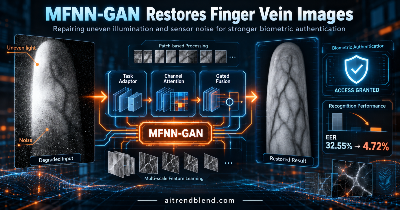
Picture a finger vein reader bolted beside a server room door. It worked flawlessly on day one. Six years later its near infrared LEDs have aged unevenly, so one side of every finger is washed out while the other sinks into shadow. The camera raises its gain to compensate, and the sensor noise rides along. Staff get rejected on the first try, then the second, and eventually someone props the door open. A team at Dongguk University in Seoul built MFNN-GAN for exactly this situation, and the question worth asking is whether software can rescue hardware that is slowly failing.
Key points
- MFNN-GAN restores finger vein images that suffer from uneven lighting and sensor noise at the same time, which earlier restoration networks did not handle.
- A small classifier called a task adaptor guesses which degradation is present and steers the restoration through channel attention.
- Gated fusion blends shallow and deep features with learned weights instead of passing them along in sequence.
- With ConvNeXt-small as the recognizer, equal error rates fell from 32.55 percent to 4.72 percent on SDUMLA-HMT-DB and from 26.2 percent to 1.73 percent on HKPU-DB.
- The restored images are not the prettiest by image quality metrics, yet they give the best recognition, and the model is slow on embedded hardware.
Why an aging illuminator wrecks recognition
Finger vein recognition works because deoxygenated hemoglobin absorbs near infrared light, which makes veins appear as dark lines inside a brighter finger. That tidy piece of physics depends on strong, even illumination. The authors of this paper, Jin Seong Hong, Seung Gu Kim, Jung Soo Kim and Kang Ryoung Park, start from a simple observation. When the illuminator ages, the light becomes both weaker and uneven, and a weak light pushes the camera sensor into a noisy regime. Two problems arrive together.
That pairing is the heart of the work. Earlier restoration research treated one villain at a time. Their own previous network, INF-GAN, normalized illumination but never saw noise during training, and its recognition performance slipped when strong noise was added. Other teams built dedicated models for motion blur and for scattering blur. Real devices rarely fail in one clean way, so a model tuned for a single fault can misfire on an image that carries two.
There is also a budget argument. Swapping the illuminator in every deployed reader costs money and downtime, and a software layer that tolerates worn hardware looks cheaper. Whether it really is cheaper depends on the compute bill, which we come back to later. The full study is open access in Engineering Applications of Artificial Intelligence and is worth reading alongside this analysis.
“The first attempt for restoring multiple degradation factors.” Hong et al., 2024, describing what MFNN-GAN contributes
What earlier work got right and where it stalled
Before restoration networks, most robustness work lived in the recognizer. Handcrafted methods such as the block averaged texture descriptor of Zhang and Wang (2022) and the anatomical vein pattern features of Krishnan and Thomas (2023) extract tidy features from tidy images. Deep recognizers are more forgiving. These include the transfer learning approach of Shaheed and colleagues (2022), the vision transformer and capsule network hybrid of Li and colleagues (2022) and the multiscale bilinear fusion of Ma and colleagues (2023). Even so, the authors argue that all of them quietly assume the input is reasonably clean.
A few older studies did face illumination and noise together. Peng and colleagues (2012) combined gray scale normalization with a Gaussian filter, and Qin and colleagues (2013) fused scores from vein shape, SIFT and orientation features. Noh and colleagues (2020) trained two DenseNet-161 networks, one on texture and one on shape, then fused their scores. Each approach stops short of repairing the image itself. When degradation is severe, simple preprocessing and score fusion cannot rebuild information that the sensor never captured cleanly.
The paper sorts prior work into three buckets, which are studies ignoring both problems, studies handling illumination only, and studies handling both. MFNN-GAN is the only entry in its comparison table that restores images under both degradations. The authors also explain why they picked a GAN over newer families. Diffusion models generate slowly because they denoise step by step, and flow based models produced lower image quality in the comparison the authors cite. A GAN generates in one pass, which matters on embedded readers. If you want a refresher on that tradeoff, our guide to GANs and diffusion models covers it.
Inside MFNN-GAN
The generator accepts a 224 by 224 region of interest cropped from the finger. A residual image generation block, inherited from INF-GAN, produces a one channel residual image that gets stacked onto the three channel input, so the network actually sees four channels. From there the path is short. There is one 7 by 7 convolution block, two down sampling blocks, four residual blocks with task channel attention, a gated fusion step, two up sampling blocks and a tanh output. The discriminator is a PatchGAN. Three ideas do the real work, and each deserves its own explanation.
The task adaptor
Think of how a dog and cat classifier behaves. Show it a dog and it reports a high probability for dog. The task adaptor does the same thing for damage. It is a trimmed down MobileNetV3 small attached after the last down sampling block, and it reports which of three degradation cases the input belongs to. The cases are a dark image with noise, a brightly saturated image, and an image with noise alone. Its output is just three numbers.
It handles its narrow job well. On SDUMLA-HMT-DB the per class accuracy ranged from 96.4 to 100 percent, and on HKPU-DB from 98.55 to 100 percent. The few mistakes came from confusing the two noisy cases with each other, which is understandable because a dark noisy finger and a merely noisy finger look alike. The catch is that the adaptor is hard wired to three labels. The authors say more degradation factors can be added as long as the matching labels are prepared, which means labeled examples and retraining.
Task channel attention
Squeeze and excitation style attention normally computes channel weights by compressing the features themselves. MFNN-GAN takes a different route. A fully connected layer stretches the three adaptor outputs to 256 values, a sigmoid squashes them between 0 and 1, and the result scales each channel of a residual block. In effect the network is told what kind of damage it is looking at and adjusts which feature channels to trust. The idea is borrowed openly from the task adaptive restoration work of Zhou and colleagues (2022), and the authors say so.
Inside each residual block sits a smooth dilated convolution. A separable convolution runs first and the dilated one follows, which softens the gridding artifacts that plain stacked dilation tends to produce. Kernel sizes grow from 3 to 7 across the first three blocks with dilation rates of 2, 3 and 4, while the fourth block falls back to a 1 by 1 kernel and a rate of 1. My reading is that the wide receptive fields help the network look past broad lighting gradients, while the small last block protects fine vein detail.
Gated fusion
Most encoder decoder restorers pass features along one stage after another, so the decoder receives whatever the last layer produced. Gated fusion changes that. The outputs of the second down sampling block and of residual blocks 1, 2 and 4 are concatenated, a single convolution turns them into weight maps, and the four features are multiplied by their weights and added together. Shallow features carry edges and blobs. Deeper ones carry vein patterns and texture. Letting the network weigh them per position and channel is more flexible than plain concatenation or summation. The paper does not explain why residual block 3 is left out of the fusion, which is a small but real open question.
Discriminator, losses and training
The PatchGAN discriminator receives seven channels, which are the four channel input plus a three channel image, and it emits a 31 by 31 map in which every element judges a 70 by 70 patch. The generator loss mixes four terms. There is the usual adversarial loss, a feature matching loss drawn from five discriminator layers, a perceptual loss from a pre trained VGG19 and the task adaptor loss. The adaptor loss is multiplied by a cosine decay so it fades as training proceeds, because a three class problem is easy and overfits fast.
Training used the Adam optimizer with a learning rate of 0.002, 130 epochs and a batch size of 1. The two weights that balance the feature matching and perceptual terms appear in the final objective, yet the text of the paper does not list their values. That matters for anyone trying to reproduce the work, and it is one reason the code later in this article marks them as placeholders.
The mathematics in plain view
Three short formulas capture most of the design. Each sits in a box below and is followed by plain language.
Task adaptor and task channel attention
$$D_f = TA(D_{out}), \qquad ResT_{out} = \mathrm{Sigmoid}\big(TCA(D_f)\big) \times ResD_{out}$$Here \(TA\) is the task adaptor and \(D_{out}\) is the final down sampling output. \(D_f\) is the three value description of the damage. \(TCA\) lifts that description to one weight per channel, and \(ResD_{out}\) is what the smooth dilated residual block produced. The product is the attended feature that moves on through the network.
Gated fusion
$$G_{fout} = G_{w1} D_{out} + G_{w2} ResT_{out1} + G_{w3} ResT_{out2} + G_{w4} ResT_{out4}$$The four weights \(G_{w1}\) to \(G_{w4}\) come from one convolution applied to the concatenated features. Each weight multiplies its own feature, and the sum becomes the input to the up sampling path.
Training objective with decayed adaptor loss
$$\max_D \min_G \; L_{GAN} + \lambda_1 L_{Feature} + \lambda_2 L_{Perceptual} + L_{TaskAdaptor}, \qquad L_{TaskAdaptor} = \frac{1+\cos(\pi \cdot epoch / P)}{2} \, \mathbb{E}\big[\lVert T(I) – L \rVert_2\big]$$The discriminator tries to maximize the adversarial term while the generator minimizes the whole sum. \(L\) is the degradation label, \(T(I)\) is the adaptor’s prediction and \(P\) is the decay period. As the epoch count approaches \(P\), the cosine factor shrinks toward zero and the adaptor loss stops dominating.
MFNN-GAN does not try to be one model that fixes everything blindly. It first diagnoses the damage with a tiny classifier, then uses that diagnosis to re weight its own feature channels.
How the degraded test data was built
The team did not collect degraded captures from aging hardware. They synthesized the damage, which is a choice worth understanding. A gamma style transform with a small 3 by 3 blur creates severely bright or dark unevenness, which is Equation 12 in the paper. A contrast adjustment then pushes the pattern closer to real uneven lighting, which is Equation 13. Gaussian noise with zero mean and a variance of 0.005 finishes the job in Equation 14. Bright images used a gain of 2.5 and an exponent of 1 on both databases. Dark images used a gain of 2 with an exponent of 0.2 on SDUMLA-HMT-DB and 0.3 on HKPU-DB.
The training mixture was 50 percent noise only, 25 percent dark with noise and 25 percent bright. SDUMLA-HMT-DB supplies 3816 images from 106 people across 636 classes, and HKPU-DB supplies 1872 images from 156 people across 312 classes. Two fold cross validation kept any class from appearing in both training and testing, and augmentation by cropping and translation grew the training images to five times their original number.
Recognition relies on a composite image trick. The enrolled image goes in channel one, the probe image in channel two, and a vertical stack of both at half height in channel three. A network then judges genuine versus impostor from how well the two align. Because small misalignments cause false rejections, inference tries nine versions, the original and eight shifted copies. One more detail changes how you should read the results. Both recognizers, DenseNet-161 and ConvNeXt-small, were trained on original undamaged images. The restorer’s job is therefore to make damaged images look like the clean ones the recognizer already knows.
What the numbers actually say
Recognition accuracy against rivals
Equal error rate, or EER, is the point where false accepts and false rejects occur equally often, so lower is better. The table below uses ConvNeXt-small as the recognizer and reproduces the paper’s reported values.
| Input or restorer | SDUMLA-HMT-DB | HKPU-DB |
|---|---|---|
| Clean originals | 0.48 | 0.25 |
| Degraded, no restoration | 32.55 | 26.2 |
| MFNN-GAN | 4.72 | 1.73 |
| CSNorm | 5.43 | 3.79 |
| NAF-Net | 5.44 | 2.43 |
| Restormer | 5.51 | 2.76 |
| PromptIR | 6.6 | 3.86 |
| Pix2Pix-HD | 6.29 | 3.52 |
| INF-GAN | 6.86 | 3.54 |
| Operation wise attention network | 11.63 | 8.13 |
| Pix2Pix | 22.67 | 14.23 |
| CycleGAN | 31.26 | 30.19 |
| EnlightenGAN | 36.16 | 29.17 |
| Attention guided image translation GAN | 37.33 | 31.41 |
Start with the anchor points. Clean originals give EERs of 0.48 and 0.25 percent. Damaged images push those to 32.55 and 26.2 percent, which is unusable. MFNN-GAN brings them back to 4.72 and 1.73 percent. That recovers most of the loss, though a gap to clean images remains, roughly four points on SDUMLA-HMT-DB and one and a half on HKPU-DB.
Among rivals, MFNN-GAN leads on both databases. The interesting detail sits one row down. The authors name NAF-Net as the second best method and test against it, yet on SDUMLA-HMT-DB the CSNorm result of 5.43 edges NAF-Net’s 5.44 by a hair. On HKPU-DB NAF-Net clearly leads the rest with 2.43. With DenseNet-161 as the recognizer, MFNN-GAN again wins at 6.33 and 2.37 against 6.73 and 3.21 for NAF-Net, but the margin on SDUMLA-HMT-DB shrinks to 0.4 points.
Restorers that made things worse
Compare three rows of the table with the degraded baseline. EnlightenGAN scored 36.16 and 29.17, the attention guided image translation GAN scored 37.33 and 31.41, and CycleGAN scored 31.26 and 30.19. Against a degraded baseline of 32.55 and 26.2, these restorers left recognition no better and usually worse. CycleGAN is unpaired, so a noisy input gets matched with an arbitrary clean target during training, which makes faithful repair hard. The authors also note that EnlightenGAN adds the input back near the end of the model, so strong noise leaks straight through. A plausible reading is that a restorer that invents believable texture can erase the thin structures identification depends on. Restoration is not automatically helpful.
The image quality paradox
Here the paper is candid. On pixel distribution measures MFNN-GAN is not the winner. Restormer posts the best FID, 8.19 on SDUMLA-HMT-DB and 12.51 on HKPU-DB, while MFNN-GAN records 15.09 and 26.63. Its d prime values of 0.15 and 0.07 and its Wasserstein distances of 2.89 and 3.22 are unremarkable, and NAF-Net sits lower on the Wasserstein distance for SDUMLA-HMT-DB at 2.71. The authors respond that these metrics compare global statistics and say little about vein structure, so they judge restoration by recognition accuracy instead. That is a fair argument for this task. It also means the honest summary is that MFNN-GAN is tuned for the recognizer and not for human eyes.
What the ablation reveals
| Task adaptor | Channel attention | Gated fusion | SDUMLA-HMT-DB | HKPU-DB |
|---|---|---|---|---|
| No | No | No | 7.55 | 2.65 |
| No | No | Yes | 6.29 | 1.98 |
| No | Yes | No | 5.81 | 1.8 |
| No | Yes | Yes | 7.77 | 1.79 |
| Yes | Yes | No | 7.16 | 2.31 |
| Yes | Yes | Yes | 4.72 | 1.73 |
The full recipe gives 4.72 and 1.73. Remove everything and you get 7.55 and 2.65. The middle rows are messier than a tidy story would like. Channel attention plus gated fusion without the adaptor reaches 1.79 on HKPU-DB but 7.77 on SDUMLA-HMT-DB, which is worse than the plain baseline. Adaptor plus attention without gated fusion gives 7.16 and 2.31. No single component carries the gain. The parts seem to help mostly in combination, which is plausible because the adaptor feeds the attention and gated fusion blends the result, yet it also makes the design harder to simplify.
The hyperparameter sweeps add a caution. Four attention blocks give 4.72 on SDUMLA-HMT-DB and 1.73 on HKPU-DB. Three blocks give 4.91 and 2.94, and five blocks give 5.54 and 2.92. For mobile bottleneck blocks inside the adaptor, two is best at 4.72 and 1.73, while one gives 8.41 and 2.18 and three gives 7.63 and 3.21. The chosen configuration sits on a sharp peak, so anyone adapting the model to new data should expect to retune.
A look inside the recognizer
The authors also compared Grad-CAM heat maps from four ConvNeXt blocks. For genuine pairs, maps from restored images highlight areas similar to maps from the original images in every block except the second, while maps from degraded images wander. Imposter pairs show the same tendency with different intensities. Heat maps are suggestive rather than conclusive, but they agree with the EER story.
Judge a restorer by the task it serves. MFNN-GAN loses on several image quality metrics and still wins on recognition, while three other GANs produced images that recognized worse than the degraded originals.
The Jetson question
Accuracy is only half of deployment. The authors timed each restorer on a desktop with an RTX 3060 and on a Jetson TX2 module, a board common in finger vein hardware. MFNN-GAN needs 25.42 ms per 224 by 224 image on the desktop and 420.33 ms on the Jetson, with 31.29 million parameters, 160.36 GFLOPs and 329.94 MB of memory. The authors call it mid tier for speed. Set against its own predecessor, INF-GAN needs 34.14 ms on the Jetson, so the new model is about twelve times slower on that board. Pix2Pix manages 13.43 ms.
Nearly half a second for restoration alone is tolerable at a door but not pleasant, and the paper does not report how long the nine way ConvNeXt matching adds on top. NAF-Net costs about the same on the Jetson at 423.51 ms, while Restormer takes 2247.38 ms. The authors list a lighter and faster model as their first piece of future work. Teams that care about this should read our notes on knowledge distillation and model compression, since distilling the generator is the obvious next step.
Do the statistics hold up
The paper runs a t test between MFNN-GAN and NAF-Net using average EER and reports a p value of 0.36 times ten to the power of minus one, which is 0.036, along with a Cohen’s d of 11.67. A d above 0.8 counts as large, so 11.67 looks overwhelming. Read it with care. The paper does not say how many independent runs fed the test, and with two databases and two fold cross validation the count cannot be large. With so few data points and tiny variance, an effect size can balloon without meaning the model is eleven standard deviations better in any practical sense. Treat it as a consistency check and not as proof of superiority. The raw EER gaps are the more honest evidence, and they favor MFNN-GAN by 0.72 points on SDUMLA-HMT-DB and 0.7 points on HKPU-DB against NAF-Net.
Where this idea fits in the bigger picture
The most transferable idea is conditioning restoration on a cheap diagnosis of the damage. All in one restoration networks such as PromptIR chase the same goal with learned prompts. MFNN-GAN does it with an explicit classifier that a practitioner can inspect and relabel. That transparency is underrated, because when a reader misbehaves in the field you can ask the adaptor what it thought it saw.
The second idea is the evaluation habit. Judging a restorer by the downstream recognizer, and not by how pleasant the picture looks, should be standard for any pipeline where a machine is the final consumer. Other near infrared biometrics such as palm vein readers face the same dim light and sensor noise, although this paper does not test them. For more restoration and synthesis work, our hub on generative AI and diffusion models collects the related analyses, and our article on image restoration networks shows how the same attention ideas appear elsewhere.
Limitations worth stating plainly
Start with data. Every degraded image in the study was manufactured with a formula, and the same team chose both the formula and the model built to undo it. Real aging hardware produces stranger patterns, and the paper never tests captures from a worn device. The noise model is Gaussian, while real sensors can show other noise behavior.
Scale comes next. Two public databases with 106 and 156 people are modest by modern biometric standards, and both contain mostly clean captures. The authors explain why they passed on MMCBNU_6000 and THU-FVFDT1, since neither suits a study of uneven lighting plus noise. The result is that generalization to other sensors, populations and finger placements remains unmeasured.
Then there is the failure the authors show themselves. In Figure 21 of the paper, enrolled and probe images from the same finger still failed to match after restoration. The degraded input was dark with strong noise, and restoration changed the composite pattern little beyond removing noise. Some information was simply gone, and no generator can invent the right vein pattern from nothing.
The rest is a short list. The adaptor is hard wired to three labeled cases, the loss weights are unreported, performance is sensitive to block counts, the model is slow on embedded hardware and the data are available only on request. We did not rerun any experiment. Everything above reflects the numbers the paper reports, and the code below is our reconstruction and not the authors’ release.
A compact PyTorch reimplementation
The listing below is our reconstruction of the architecture and training step, written from the paper’s tables and equations. It is not the authors’ release, which they point to on GitHub. Where the paper leaves a detail open, a comment in the code says what was assumed. The loss weights of 10 are placeholders, the degradation function follows our reading of Equations 12 to 14, and the smoke test at the bottom runs two training steps on random tensors, which is meant to confirm that shapes line up and not to reproduce any result.
"""
MFNN-GAN reference implementation (PyTorch).
Re-implementation written from the description in Hong et al., 2024 (Engineering
Applications of Artificial Intelligence 133, 108036). It is NOT the authors' code.
Where the paper leaves a detail open, a comment says what was assumed.
"""
import math
import torch
import torch.nn as nn
import torch.nn.functional as F
import torchvision


# ---------------------------------------------------------------- basic blocks
class ConvBlock(nn.Module):
    """Conv, ReLU, instance norm (the 'Conv block' of Table 2)."""
    def __init__(self, cin, cout, k=3, s=1, p=1):
        super().__init__()
        self.body = nn.Sequential(
            nn.Conv2d(cin, cout, k, s, p), nn.ReLU(True), nn.InstanceNorm2d(cout))

    def forward(self, x):
        return self.body(x)


class ResidualImageBlock(nn.Module):
    """RIGB from INF-GAN. Layer counts follow Table 2, exact ordering is assumed."""
    def __init__(self):
        super().__init__()
        layers = [nn.Conv2d(3, 64, 3, padding=1), nn.ReLU(True)]
        for _ in range(2):
            layers += [nn.Conv2d(64, 64, 1), nn.ReLU(True)]
        for _ in range(3):
            layers += [nn.Conv2d(64, 64, 3, padding=1), nn.ReLU(True)]
        layers += [nn.Conv2d(64, 1, 1)]
        self.body = nn.Sequential(*layers)

    def forward(self, x):
        return self.body(x)


# ------------------------------------------------------------- task adaptor
class SqueezeExcite(nn.Module):
    def __init__(self, ch, r=4):
        super().__init__()
        self.fc = nn.Sequential(nn.AdaptiveAvgPool2d(1), nn.Conv2d(ch, ch // r, 1),
                                nn.ReLU(True), nn.Conv2d(ch // r, ch, 1), nn.Hardsigmoid())

    def forward(self, x):
        return x * self.fc(x)


class MobileBottleneck(nn.Module):
    """Expand, depthwise conv, squeeze excite, project (MobileNetV3 style)."""
    def __init__(self, cin, cexp, cout, k=5, stride=2):
        super().__init__()
        self.expand = nn.Sequential(nn.Conv2d(cin, cexp, 1), nn.Hardswish())
        self.dw = nn.Sequential(
            nn.Conv2d(cexp, cexp, k, stride, k // 2, groups=cexp), nn.Hardswish())
        self.se = SqueezeExcite(cexp)
        self.project = nn.Conv2d(cexp, cout, 1)

    def forward(self, x):
        return self.project(self.se(self.dw(self.expand(x))))


class TaskAdaptor(nn.Module):
    """Small MobileNetV3 style classifier that predicts the degradation type."""
    def __init__(self, cin=256, n_cls=3):
        super().__init__()
        self.b1 = MobileBottleneck(cin, 576, 48)
        self.b2 = MobileBottleneck(48, 576, 96)
        self.head = nn.Sequential(
            nn.Conv2d(96, 576, 1), nn.Hardswish(), nn.AdaptiveAvgPool2d(1),
            nn.Conv2d(576, 1024, 1), nn.Hardswish(), nn.Flatten(), nn.Linear(1024, n_cls))

    def forward(self, x):
        return self.head(self.b2(self.b1(x)))


# ------------------------------------------- residual block with task attention
class SmoothDilatedConv(nn.Module):
    """Separable conv first, then dilated conv, to soften gridding artifacts.
    The original shared convolution is approximated by a depthwise plus pointwise pair."""
    def __init__(self, ch, k, rate):
        super().__init__()
        self.ss = nn.Sequential(nn.Conv2d(ch, ch, k, padding=k // 2, groups=ch),
                                nn.Conv2d(ch, ch, 1))
        self.dil = nn.Conv2d(ch, ch, 3, padding=rate, dilation=rate)

    def forward(self, x):
        return self.dil(self.ss(x))


class TaskChannelResBlock(nn.Module):
    """ResT = sigmoid(TCA(Df)) * ResD(x), then added back to the input."""
    def __init__(self, ch, k, rate):
        super().__init__()
        self.body = nn.Sequential(
            SmoothDilatedConv(ch, k, rate), nn.InstanceNorm2d(ch), nn.ReLU(True),
            SmoothDilatedConv(ch, k, rate), nn.InstanceNorm2d(ch))
        self.tca = nn.Linear(3, ch)  # lifts the 1x1x3 adaptor output to one weight per channel

    def forward(self, x, df):
        w = torch.sigmoid(self.tca(df))[:, :, None, None]
        return x + w * self.body(x)


class GatedFusion(nn.Module):
    """One conv predicts a weight map for each of four features, then a weighted sum."""
    def __init__(self, ch=256, n=4):
        super().__init__()
        self.n = n
        self.gate = nn.Conv2d(ch * n, ch * n, 3, padding=1)

    def forward(self, feats):
        weights = torch.chunk(self.gate(torch.cat(feats, 1)), self.n, 1)
        return sum(w * f for w, f in zip(weights, feats))


# ----------------------------------------------------------------- generator
class Generator(nn.Module):
    def __init__(self, base=64, n_cls=3):
        super().__init__()
        ch = base * 4
        self.rigb = ResidualImageBlock()
        self.conv_in = ConvBlock(4, base, 7, 1, 3)
        self.down1 = ConvBlock(base, base * 2, 3, 2, 1)
        self.down2 = ConvBlock(base * 2, ch, 3, 2, 1)
        self.adaptor = TaskAdaptor(ch, n_cls)
        # (separable kernel, dilation rate) per block, read from Table 4
        cfg = [(3, 2), (5, 3), (7, 4), (1, 1)]
        self.res = nn.ModuleList([TaskChannelResBlock(ch, k, r) for k, r in cfg])
        self.fusion = GatedFusion(ch, 4)
        self.up1 = nn.Sequential(nn.ConvTranspose2d(ch, base * 2, 3, 2, 1, output_padding=1),
                                 nn.ReLU(True), nn.InstanceNorm2d(base * 2))
        self.up2 = nn.Sequential(nn.ConvTranspose2d(base * 2, base, 3, 2, 1, output_padding=1),
                                 nn.ReLU(True), nn.InstanceNorm2d(base))
        self.out = nn.Sequential(nn.Conv2d(base, 3, 7, 1, 3), nn.Tanh())

    def forward(self, x):
        inp = torch.cat([x, self.rigb(x)], 1)          # 4 channel input
        d2 = self.down2(self.down1(self.conv_in(inp)))
        logits = self.adaptor(d2)
        df = F.softmax(logits, 1)                        # degradation information Df
        r1 = self.res[0](d2, df)
        r2 = self.res[1](r1, df)
        r3 = self.res[2](r2, df)
        r4 = self.res[3](r3, df)
        fused = self.fusion([d2, r1, r2, r4])            # block 3 is skipped, as in Eq. 5
        return self.out(self.up2(self.up1(fused))), logits, inp


# ------------------------------------------------------------- discriminator
class PatchDiscriminator(nn.Module):
    """70x70 PatchGAN. Input is the 4 channel input plus a 3 channel image."""
    def __init__(self, cin=7):
        super().__init__()

        def blk(i, o, s):
            return nn.Sequential(nn.Conv2d(i, o, 4, s, 2), nn.LeakyReLU(0.2, True),
                                 nn.InstanceNorm2d(o))

        self.blocks = nn.ModuleList([
            nn.Sequential(nn.Conv2d(cin, 64, 4, 2, 2), nn.LeakyReLU(0.2, True)),
            blk(64, 128, 2), blk(128, 256, 2), blk(256, 512, 1),
            nn.Sequential(nn.AvgPool2d(3, 1, 1), nn.Conv2d(512, 1, 4, 1, 2))])

    def forward(self, x):
        feats = []
        for b in self.blocks:
            x = b(x)
            feats.append(x)
        return x, feats  # patch logits and five feature maps for feature matching


# -------------------------------------------------------------------- losses
def adversarial_loss(logits, real):
    target = torch.ones_like(logits) if real else torch.zeros_like(logits)
    return F.binary_cross_entropy_with_logits(logits, target)


def feature_matching_loss(f_fake, f_real):
    return sum(F.l1_loss(a, b.detach()) for a, b in zip(f_fake, f_real)) / len(f_fake)


class PerceptualLoss(nn.Module):
    """L1 distance between VGG19 features. Pass pretrained=True for real training."""
    def __init__(self, pretrained=False):
        super().__init__()
        w = torchvision.models.VGG19_Weights.IMAGENET1K_V1 if pretrained else None
        vgg = torchvision.models.vgg19(weights=w).features.eval()
        for p in vgg.parameters():
            p.requires_grad_(False)
        cuts = [2, 7, 12, 21, 30]
        self.slices = nn.ModuleList(
            [vgg[a:b] for a, b in zip([0] + cuts[:-1], cuts)])
        self.register_buffer("mean", torch.tensor([0.485, 0.456, 0.406]).view(1, 3, 1, 1))
        self.register_buffer("std", torch.tensor([0.229, 0.224, 0.225]).view(1, 3, 1, 1))

    def forward(self, a, b):
        a = ((a + 1) / 2 - self.mean) / self.std
        b = ((b + 1) / 2 - self.mean) / self.std
        loss = 0.0
        for s in self.slices:
            a, b = s(a), s(b)
            loss = loss + F.l1_loss(a, b)
        return loss


def task_adaptor_loss(logits, labels, epoch, period):
    """Eq. 10. Cosine decay keeps the easy classifier from overfitting."""
    decay = 0.5 * (1 + math.cos(math.pi * epoch / period))
    onehot = F.one_hot(labels, logits.size(1)).float()
    return decay * F.mse_loss(F.softmax(logits, 1), onehot)


# ------------------------------------------------------------ training step
def train_step(G, D, perc, opt_g, opt_d, clean, degraded, labels, epoch,
               lam1=10.0, lam2=10.0, period=130):
    """lam1 and lam2 are not reported in the paper. These defaults are placeholders."""
    restored, logits, inp = G(degraded)
    real_pair = torch.cat([inp.detach(), clean], 1)

    # discriminator update
    opt_d.zero_grad()
    d_real, _ = D(real_pair)
    d_fake, _ = D(torch.cat([inp.detach(), restored.detach()], 1))
    loss_d = 0.5 * (adversarial_loss(d_real, True) + adversarial_loss(d_fake, False))
    loss_d.backward()
    opt_d.step()

    # generator update
    opt_g.zero_grad()
    d_fake, f_fake = D(torch.cat([inp, restored], 1))
    with torch.no_grad():
        _, f_real = D(real_pair)
    loss_g = (adversarial_loss(d_fake, True)
              + lam1 * feature_matching_loss(f_fake, f_real)
              + lam2 * perc(restored, clean)
              + task_adaptor_loss(logits, labels, epoch, period))
    loss_g.backward()
    opt_g.step()
    return loss_d.item(), loss_g.item()


# -------------------------------------------------- synthetic degradation data
def degrade(gray, case, dataset="sdumla"):
    """Eqs. 12 to 14. gray is (B,1,H,W) in [0,1]. case is noise, dark or bright.
    How Eq. 13 applies to the bright case is not spelled out, so it is skipped here."""
    x = gray
    if case in ("dark", "bright"):
        a, beta = (2.5, 1.0) if case == "bright" else (2.0, 0.2 if dataset == "sdumla" else 0.3)
        k = torch.tensor([1.0, 2.0, 1.0])
        k = (k[:, None] * k[None, :] / 16).view(1, 1, 3, 3).to(gray)
        x = F.conv2d(a * gray.clamp_min(1e-6) ** beta, k, padding=1)     # Eq. 12
        if case == "dark":
            x = 2 * x.mean((2, 3), keepdim=True).expand_as(x) - x          # Eq. 13
            lo, hi = x.amin((2, 3), keepdim=True), x.amax((2, 3), keepdim=True)
            x = (x - lo) / (hi - lo + 1e-8)
    if case in ("noise", "dark"):
        x = x + math.sqrt(0.005) * torch.randn_like(x)                     # Eq. 14
    return x.clamp(0, 1)


# ---------------------------------------------------------------- evaluation
@torch.no_grad()
def evaluate_restoration(G, loader, device="cpu"):
    """Mean L1 error and PSNR between restored and clean images (range [-1,1])."""
    G.eval()
    l1s, psnrs = [], []
    for degraded, clean in loader:
        restored, _, _ = G(degraded.to(device))
        clean = clean.to(device)
        l1s.append(F.l1_loss(restored, clean).item())
        mse = F.mse_loss((restored + 1) / 2, (clean + 1) / 2).item()
        psnrs.append(10 * math.log10(1.0 / max(mse, 1e-10)))
    G.train()
    return sum(l1s) / len(l1s), sum(psnrs) / len(psnrs)


def compute_eer(genuine, impostor):
    """Equal error rate in percent. Higher score means more likely genuine."""
    thresholds = torch.unique(torch.cat([genuine, impostor]))
    best_gap, best_eer = 1e9, 100.0
    for t in thresholds:
        frr = (genuine < t).float().mean().item()
        far = (impostor >= t).float().mean().item()
        if abs(far - frr) < best_gap:
            best_gap, best_eer = abs(far - frr), 100 * (far + frr) / 2
    return best_eer


# ----------------------------------------------------------------- smoke test
if __name__ == "__main__":
    torch.manual_seed(0)
    G, D = Generator(), PatchDiscriminator()
    perc = PerceptualLoss(pretrained=False)   # random weights keep the test offline
    opt_g = torch.optim.Adam(G.parameters(), lr=0.002, betas=(0.9, 0.99))
    opt_d = torch.optim.Adam(D.parameters(), lr=0.002, betas=(0.9, 0.99))

    gray = torch.rand(2, 1, 64, 64)                        # dummy vein images
    cases = ["dark", "bright"]
    degraded = torch.cat([degrade(gray[i:i + 1], c) for i, c in enumerate(cases)])
    degraded = degraded.repeat(1, 3, 1, 1) * 2 - 1
    clean = gray.repeat(1, 3, 1, 1) * 2 - 1
    labels = torch.tensor([0, 1])

    for epoch in range(2):
        ld, lg = train_step(G, D, perc, opt_g, opt_d, clean, degraded, labels, epoch)
        print(f"epoch {epoch}  D loss {ld:.3f}  G loss {lg:.3f}")

    restored, logits, _ = G(degraded)
    print("restored", tuple(restored.shape), "adaptor logits", tuple(logits.shape))
    print("L1 and PSNR", evaluate_restoration(G, [(degraded, clean)]))
    print("EER on random scores", compute_eer(torch.rand(50) + 0.3, torch.rand(500)))
Conclusion
MFNN-GAN shows that a finger vein reader with dim, uneven light and a noisy sensor can be rescued in software. On ConvNeXt-small the equal error rate drops from 32.55 to 4.72 percent on SDUMLA-HMT-DB and from 26.2 to 1.73 percent on HKPU-DB. It beats all eleven competing restorers on both databases, and it does so again with DenseNet-161 as the recognizer. For a method aimed at keeping deployed hardware useful, that is a meaningful result.
The conceptual shift is worth more than the benchmark. Most restoration models behave as if the job is always the same. This one diagnoses first and acts second. A tiny classifier names the damage, and that name reshapes the feature channels inside the generator. Gated fusion then lets the network decide how much to trust shallow edges against deeper vein structure. Neither idea is exotic, yet the combination is well matched to a problem where damage comes in combinations.
The approach should transfer to any imaging pipeline with a small number of known failure modes. Other near infrared biometrics, industrial inspection cameras and low light sensors come to mind. That is a hypothesis and not a finding, because the paper tests only finger veins. The effort needed is also concrete, since each new failure mode needs labeled examples and a retrained adaptor.
The limits deserve as much attention as the gains. The damage was synthetic, the adaptor knows only three cases, the best configuration sits on a narrow peak, a dark and noisy capture still defeated the system in the authors’ own failure figure, and clean images remain clearly better than restored ones. On a Jetson TX2 the model takes 420.33 ms per image, roughly twelve times longer than INF-GAN. A worn reader repaired by software is still a worn reader.
The authors name their next steps plainly. They want a lighter and faster model, a recognition method that survives low illumination with strong noise, and support for more degradation factors. They also suggest unsupervised learning so the system can adapt to damage nobody labeled, and they propose trying the idea on images other than finger veins. To that list we would add testing on captures from genuinely aged devices and distilling the generator for embedded boards.
A reader that can tell what is wrong with its own eyesight before it tries to see is a better reader, and that may be the most useful idea in this paper.
Frequently asked questions
What is MFNN-GAN?
MFNN-GAN is a generative adversarial network from Dongguk University that restores finger vein images damaged by uneven illumination and sensor noise at the same time. It is built so that recognition still works when the near infrared illuminator of a reader is weak or unbalanced.
How does the task adaptor help?
The task adaptor is a small classifier that labels the damage as dark with noise, bright saturation or noise alone. Its output becomes channel attention weights inside the residual blocks, so the restoration adapts to the kind of damage found in each image.
How much does MFNN-GAN improve recognition?
With ConvNeXt-small as the recognizer, the equal error rate fell from 32.55 percent to 4.72 percent on SDUMLA-HMT-DB and from 26.2 percent to 1.73 percent on HKPU-DB. Clean images still score better at 0.48 and 0.25 percent.
Can MFNN-GAN run on an embedded reader?
It can run, but slowly. The paper reports 420.33 ms per image on a Jetson TX2 module against 25.42 ms on a desktop with an RTX 3060, and the authors list a lighter model as future work.
Is the code available?
The authors point to a public GitHub repository named MFNN-GAN and state that the data will be made available on request. This article also includes our own reconstruction of the architecture for study purposes.
Does it remove the need to replace a failing illuminator?
Not entirely. It reduces the damage from a weak or uneven illuminator, yet the paper shows a failure case with dark images and strong noise, and it tests only synthetic degradation. Treat it as a way to extend the life of a reader and not as a license to ignore failing hardware.
Read the source and explore the code
The paper is open access, and the authors published their implementation.
Read the paper View the authors’ codeHong, J.S., Kim, S.G., Kim, J.S., Park, K.R., 2024. Deep learning-based restoration of multi-degraded finger-vein image by non-uniform illumination and noise. Engineering Applications of Artificial Intelligence 133, 108036. https://doi.org/10.1016/j.engappai.2024.108036
This analysis is based on the published paper and an independent evaluation of its claims.