What is a factorizable density?

It is a density that can be written as a product of smaller functions, each depending on only a few of the variables. Bayesian networks and Markov random fields are the standard examples. The size of the largest group of variables is the effective dimension, written d.

What does minimax optimal up to logarithmic factors mean here?

It means no estimator can beat the stated rate in the worst case over the whole family of densities, and the diffusion estimator matches that rate apart from powers of the logarithm of n. Those logarithmic powers are the price the proof pays.

Does the paper prove that diffusion models escape the curse of dimensionality?

No. It proves a rate that depends on the effective dimension for factorizable densities, with a fixed ambient dimension and several technical assumptions. The ambient dimension still appears in the logarithmic factors and in the constants.

Are sparse weight sharing networks required?

The evidence says no. A concurrent preprint by Fan, Gu and Li reaches the same result with fully connected networks, and the authors' experiments show both architectures performing about the same. The authors say openly that they have not shown a distinct advantage.

Why did the experiments use Wasserstein distance and not total variation?

Total variation needs an explicit density estimate, and a diffusion model only provides samples. The authors therefore compared sample sets with the Wasserstein 1 distance, computed through Sinkhorn iterations.

How many samples does a diffusion model need according to this paper?

The paper gives no sample size recipe. In its five dimensional simulations, models trained on 500 samples beat a kernel estimator trained on 100,000 in the two settings with richer dependence, but those are synthetic data and the result may not transfer to real datasets.

Diffusion Models and Factorizable Density Estimation

Analysis by the aitrendblend editorial team · Based on Kwon, Kim, Ohn and Chae, JMLR 27 (2026) · 5 October 2026

diffusion models
density estimation
minimax optimality
score matching
Markov random fields
weight sharing networks

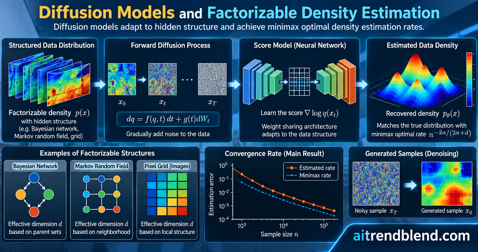
Diffusion model density estimation with a sparse weight sharing score network, illustrating factorizable density estimation from the 2026 JMLR paper by Kwon, Kim, Ohn and Chae — Feature illustration. A diffusion model turns noise into samples, and the paper asks how fast the implied density estimate converges.

Picture a table with five columns and five hundred rows. The columns lean on each other in a chain, so column two says a lot about column three and very little about column five. You want a model of the whole joint distribution. A kernel density estimator will give you one, and it will want an uncomfortable number of rows before the result stops being poor. In the simulations behind a new JMLR paper, a diffusion model trained on just five hundred such rows beat a kernel estimator that was handed one hundred thousand. Why that can happen is the question the paper sets out to answer.

Key points

The paper treats a diffusion model as a density estimator and asks how quickly its implied estimate converges to the truth.
If the density factorizes into pieces that each touch at most $d$ variables, the estimator reaches the rate $n^{-\beta/(2\beta+d)}$ in total variation distance, which is minimax optimal up to logarithmic factors.
The estimator is never told the factorization, yet it adapts to it. That adaptivity is the real contribution.
The proof uses sparse weight sharing networks, and convolutions are a special case. A concurrent preprint gets the same rate with fully connected networks, so the architecture is a proof device and not a proven advantage.
In simulations with five dimensional data, diffusion models beat kernel density estimation in every setting and beat a two stage deep baseline when the dependence was richer.
The theory assumes bounded support, a density bounded away from zero, and a fixed dimension, and the logarithmic factors grow with that dimension.

The question behind the paper

Diffusion models are famous for pictures, audio and video. Statisticians ask something plainer. Strip away the artistry, treat the model as a machine that turns $n$ samples into an estimate of a probability density, and measure how good that machine is. Then ask why it keeps working in dimensions where the classical tools fall apart.

The classical picture is bleak. Take a density in $D$ dimensions with smoothness measured by a Hölder exponent $\beta$. The best achievable error in total variation distance shrinks like $n^{-\beta/(D+2\beta)}$, a result the authors credit to Tsybakov (2008) and Giné and Nickl (2016). Look at where $D$ sits. It is in the denominator of the exponent, so every extra variable slows learning, and a modest image has hundreds of pixels.

Real data rarely uses all those dimensions freely. Hyeok Kyu Kwon, Dongha Kim, Ilsang Ohn and Minwoo Chae, working at POSTECH, Sungshin Women’s University and Inha University, pick one specific kind of hidden simplicity and ask whether a diffusion model can find it unaided. The simplicity is factorization. They assume the density splits into a product of smaller functions.

$$p_0(\mathbf{x})=\prod_{I\in\mathcal{I}} g_I(\mathbf{x}_I),\qquad d=\max_{I\in\mathcal{I}}|I|$$

Equation 1. The factorization assumption and the effective dimension

Each factor $g_I$ looks only at the coordinates listed in the index set $I$, and $d$ is the size of the biggest set. When $d$ is far below $D$, classical theory says the rate improves to $n^{-\beta/(2\beta+d)}$. Building an estimator with that rate is easy when the factorization is known in advance. The hard version, and the one this paper takes on, is an estimator that does not know the factorization and still reaches the rate.

Where factorization shows up

The assumption sounds abstract until you see how many familiar models satisfy it. A Bayesian network writes the density as a product of conditionals, one per variable given its parents, so the effective dimension is one plus the largest number of parents. A Markov random field gives a product over maximal cliques through the Hammersley and Clifford theorem, so $d$ is the size of the largest clique. The authors draw a seven variable example of each in Figure 2 of the paper, with $d=4$ for the directed graph and $d=3$ for the undirected one. For a hands on look at the conditional independence machinery behind such graphs, see our explainer on how conditioning rewires a causal Bayesian network.

Images are where this gets interesting. Neighboring pixels move together and distant ones barely notice each other, which is exactly the local Markov property. Figure 3 of the paper shows a handwritten digit with two candidate pixel graphs. A plain grid gives $d=2$, and adding diagonal neighbors gives $d=4$. Either way $d$ stays tiny next to the number of pixels. If you want the wider context on how diffusion models are used, our Generative & Diffusion Models archive collects the practical coverage.

How the estimator is built

The construction follows the standard diffusion recipe, which is worth restating because the theory lives in the details. A forward process gradually blurs the data into Gaussian noise using an Ornstein Uhlenbeck type equation.

$$d\mathbf{X}_t=-\alpha_t\mathbf{X}_t\,dt+\sqrt{2\alpha_t}\,d\mathbf{B}_t,\qquad \mathbf{X}_0\sim P_0$$

Equation 2. The forward process

Because the process is linear, the conditional law of $\mathbf{X}_t$ given $\mathbf{X}_0=\mathbf{x}_0$ is Gaussian with mean $\mu_t\mathbf{x}_0$ and variance $\sigma_t^2$, where $\mu_t=\exp(-\int_0^t\alpha_s\,ds)$ and $\sigma_t^2=1-\mu_t^2$. Anderson (1982) showed that running the process backwards in time gives another diffusion. Its drift contains the score function $\nabla\log p_t$, the gradient of the log density of the noised data. Learn the score at every noise level and you can start from pure noise and walk back to something that looks like data.

Learning the score uses denoising score matching in the form popularized by Vincent (2011). The training loss compares the network output with a quantity that depends only on the clean sample, the noisy sample and the known noise level.

$$\min_{\mathbf f\in\mathcal F}\ \frac1n\sum_{i=1}^{n}\int_{\underline T}^{\overline T}\lambda_t\,\mathbb{E}\Big[\Big\|\mathbf f(\mathbf X_t,t)+\frac{\mathbf X_t-\mu_t\mathbf x_0}{\sigma_t^2}\Big\|_2^2\ \Big|\ \mathbf X_0=\mathbf X^i\Big]\,dt$$

Equation 3. The empirical risk minimization problem

Two details matter. The integral stops short of zero, at a lower time $\underline T=n^{-\tau_{\min}}$, because the score blows up as the noise vanishes. It also stops at an upper time $\overline T=\tau_{\max}\log n$, long enough for the forward process to forget the data. Both choices are tied to the sample size, and they are part of what the theorem controls.

Now the subtle part. Nobody ever writes down a density estimate. The estimator $\widehat p$ is the law of a sample produced by the reverse process, which starts at a standard Gaussian and uses the learned score as its drift.

$$d\widehat{\mathbf Y}_t=\Big[\alpha_{\overline T-t}\widehat{\mathbf Y}_t+2\alpha_{\overline T-t}\,\widehat{\mathbf f}(\widehat{\mathbf Y}_t,\overline T-t)\Big]dt+\sqrt{2\alpha_{\overline T-t}}\,d\mathbf B_t,\qquad \widehat{\mathbf Y}_0\sim\mathcal N(\mathbf 0,\mathbb I_D)$$

Equation 4. The reverse process that defines the implicit estimator

So the object under study is a distribution you can sample from and never evaluate, which is why proving things about it takes real work. One caveat appears in the authors’ Remark 2. The theory ignores the error from discretizing this equation on a computer, for instance with the Euler Maruyama scheme. The authors argue the results survive a sufficiently fine time grid, and they point to Oko et al. (2023) for how that error can be handled.

The assumptions worth reading before you quote the result

A theorem is only as portable as its hypotheses. The table below lists the ones that do the heavy lifting.

Table 1. The main assumptions behind Theorem 3
Label	What it says	Why it is there
S, structure and smoothness	The density factorizes as in Equation 1, and both the density and every factor are $\beta$ Hölder smooth on the cube $[-1,1]^D$.	This is the structural premise the whole result rests on.
L, lower bound	The density is at least a positive constant $\tau_1$ everywhere on the cube.	It keeps the score, a ratio of gradient to density, well defined. The authors call it a technical convenience, following Oko et al. (2023).
B, boundary	Derivatives of the density stay bounded near the edge of the cube.	It tames the awkward boundary behavior that L creates.
Data and schedule	Samples are i.i.d. on the cube, and $\alpha_t$ stays between two positive constants with bounded derivatives.	It covers the standard choice $\alpha_t=1$ and the linear schedules used in DDPM.

Assumption L has an uncomfortable side effect. A density bounded away from zero on a cube cannot also be smooth across the edge of that cube, because it has to drop to zero outside. That forces extra care at the boundary, which is the job of assumption B. The authors note that Fan et al. (2025) obtain similar results without B, and that their approach could in principle be adapted to remove B from this framework as well.

The main result in plain language

Here is Theorem 3 stripped to its message. With a suitable class of networks, the expected total variation distance between the true density and the diffusion estimator is bounded by a quantity $\epsilon_n$.

$$\mathbb{E}\big[d_{\mathrm{TV}}(p_0,\widehat p)\big]\le\epsilon_n,\qquad \epsilon_n=C_1\,n^{-\frac{\beta}{2\beta+d}}\Big\{(\log n)^{2D+2\beta+1}+(\log n)^{10}\Big\}$$

Equation 5. The convergence rate of the diffusion estimator

Read the exponent first. It contains $d$, the effective dimension, and not $D$. Then compare it with the lower bound, which the authors lift from the classical result of Giné and Nickl (2016). No estimator, however clever, can beat $n^{-\beta/(2\beta+d)}$ uniformly over the class of factorizable densities with smooth factors.

$$\inf_{\widehat p}\ \sup_{p_0\in\mathcal G(\beta,D,d,K)}\mathbb{E}\big[d_{\mathrm{TV}}(p_0,\widehat p)\big]\ \gtrsim\ n^{-\beta/(2\beta+d)}$$

Equation 6. The minimax lower bound

The upper and lower bounds meet, apart from the logarithm. That is what minimax optimal up to logarithmic factors means. The estimator is as good as anything can be in the worst case over this family, give or take a polylogarithmic penalty.

That penalty deserves a second look. The exponent on $\log n$ contains $2D+2\beta+1$, so it grows with the ambient dimension. For moderate $n$ a large power of a logarithm can swamp the polynomial gain, and the constant $C_1$ hides further dependence on $D$ and $\beta$. The theorem is an asymptotic statement. It tells you which way the curve bends and says nothing about where it crosses the curves of competing methods.

What adaptivity means here

The architecture in Theorem 3, including depth, width, sparsity and the permutation matrices, depends on the data only through the ratio $\beta/d$ and on known constants. Nobody supplies the index sets $\mathcal I$. The network is built for a smoothness and an effective dimension, and it then handles whichever factorization the data happens to have. In that sense the estimator adapts to the structure.

The authors are careful about the limits of this claim. They state that they do not construct a fully adaptive estimator, because the hyperparameters still depend on $\beta/d$. They also remind readers that practical networks are far more elaborate and carefully tuned than the ones in the proof.

To feel the size of the gain, plug numbers into the exponent. The table below is our own arithmetic from the formulas in the paper, with $D=5$ to match the experiments, and it is not a set of results the authors report.

Table 2. Rate exponent $\beta/(2\beta+d)$ for D equal to 5 (our arithmetic from the paper’s formula)
Effective dimension	Exponent for $\beta=1/2$	Exponent for $\beta=2$
$d=1$	$1/4$	$2/5$
$d=2$	$1/6$	$1/3$
$d=5$, no structure	$1/12$	$2/9$

The last row reproduces the classical exponent $\beta/(D+2\beta)$, since $d=D$ there. Going from no structure to $d=2$ triples the exponent when $\beta=1/2$ and raises it from $2/9$ to $1/3$ when $\beta=2$. Those are the kinds of gaps that can turn an impossible sample size requirement into a feasible one.

Key takeaway

The headline is not that diffusion models are good at density estimation. It is that the same estimator reaches the optimal rate for whatever factorization the data has, without being told where the structure sits.

“Diffusion models can adapt not only to this structure but also to other structures discussed above, making them significantly more practical alternatives.”
Kwon, Kim, Ohn and Chae, JMLR 27 (2026), on estimators that adapt to factorization only

Why the proof needs sparse weight sharing networks

The authors do not use plain feedforward networks. They define a class where weights are both sparse and reused, and they write each layer with permutation matrices that decide where the shared blocks go.

$$\mathbf f_i(\cdot)=\rho\Big(\sum_{j=1}^{m_i}R_i^{(j)}\big(W_iQ_i^{(j)}\,\cdot+\mathbf b_i\big)\Big),\qquad \sum_{i}\big(\|W_i\|_0+\|\mathbf b_i\|_0\big)\le s$$

Equation 7. One layer of a sparse weight sharing network

Think of the permutation matrices $Q$ and $R$ as a way of dropping one small block of weights into many places. A convolution is the textbook case. Flatten a four by four image, slide a two by two filter over it, and the operation becomes a nine by sixteen matrix. Most entries are zero and the same four filter weights repeat in every row, as the authors show in Figure 1 of the paper. Sparse because the zeros dominate, shared because the same numbers recur. That is the reason convolutional and recurrent networks, which dominate diffusion practice, count as special cases.

The hardest step in the proof is approximating the score of the noised density $p_t$, which is defined through a $D$ dimensional integral. A standard $D$ dimensional quadrature rule needs on the order of $\epsilon^{-D/\beta}$ nodes for accuracy $\epsilon$, far too many for a network to represent. The authors take a different route. They apply a one dimensional $m$ point quadrature rule once in each of the $D$ coordinates. That still produces $m^D$ terms, but each weight is a product of $D$ numbers drawn from only $m$ distinct values, and one function $g$ is evaluated at all the nodes. Weight sharing lets the network pay for roughly $m$ distinct parameters, up to polylogarithmic factors, instead of $m^D$.

They also split the space of inputs and times into four regions. Far outside the support the density is nearly zero. At large times it is very smooth. Near the boundary assumption B helps. The interior at small times is the hard case, and that is where the quadrature trick lives. The payoff is Theorem 5, which bounds the approximation error of the score by $m^{-2\beta/d}$ times a power of $\log m$, using a network whose sparsity grows only linearly in $m$ up to logarithmic factors.

$$\inf_{\mathbf f\in\mathcal F_{\mathrm{WSNN}}\cap\mathcal F_\infty}\int_{\underline T}^{\overline T}\!\!\int_{\mathbb R^D}\|\mathbf f_0-\mathbf f\|_2^2\,p_t\,d\mathbf x\,dt\ \lesssim\ m^{-2\beta/d}(\log m)^{4D+4\beta+1}$$

Equation 8. The score approximation bound of Theorem 5

Is sparse weight sharing actually necessary?

Here the authors are refreshingly direct. While finalizing their revision they learned of a preprint by Fan, Gu and Li (2025), available as arXiv 2510.03994, that studies essentially the same problem, with the same assumption and the same rate. The difference is the architecture, since Fan and coauthors use fully connected networks. The Kwon team concedes that their results therefore do not demonstrate a distinct theoretical advantage of weight sharing.

Their experiments agree. Across all settings, diffusion models with fully connected networks performed about as well as those with weight sharing. The authors still suspect that sparse weight sharing approximates certain function classes more efficiently, and they flag that as a worthwhile direction for future work.

Table 3. The two score networks compared in the simulations
Network	Blocks	Layer type	Parameters	Learning rate
DDPM with WSNN	9	Conv1D, kernel size 11, padding 5, on a 160 dimensional feature	265,483	$5\times10^{-3}$
DDPM with FCNN	3	Dense layers of size 160 by 160	260,485	$10^{-3}$

I read this episode as a point in the paper’s favor. A theory paper can adopt a convenient architecture to push a proof through without claiming the architecture explains why the method works. The authors say so plainly, and readers should hold them to that reading.

If you are curious how sparsity shows up inside real diffusion architectures, our analysis of Salad and its sparse denoising for protein design is a good companion.

Why vanilla score matching probably is not enough

Before diffusion models took over, score matching meant estimating the single score $\nabla\log p_0$ with the loss of Hyvärinen (2005), which contains the trace of the network’s Jacobian. A sampler based on Langevin dynamics then turns the learned score into a density estimator, call it $\widehat p_{\mathrm{VS}}$. The trace term is already a practical headache in high dimensions, which is part of why the approach is rarely used for large problems.

The authors go further and conjecture that $\widehat p_{\mathrm{VS}}$ cannot reach the optimal rate even if it were computationally cheap. The reason is smoothness. The score of a $\beta$ smooth density is only $(\beta-1)$ smooth, and the best possible rate for estimating the score is therefore slower.

$$\inf_{\widehat{\mathbf f}}\ \sup_{p_0\in\mathcal G(\beta,D,d,K)}\mathbb{E}\Big[\big\|\widehat{\mathbf f}(\mathbf X_0)-\nabla\log p_0(\mathbf X_0)\big\|_2\Big]\ \gtrsim\ n^{-\frac{\beta-1}{2\beta+d}}$$

Equation 9. The lower bound for estimating a single score function

A quick calculation shows the size of the gap. With $\beta=2$ and $d=2$, the density rate exponent is $1/3$ while the score rate exponent is $1/6$. Through Girsanov’s theorem the slower score rate transfers to the density estimator built on it. The authors are explicit that the final step is a conjecture, and they do not prove that $d_{\mathrm{TV}}(\widehat p_{\mathrm{VS}},p_0)$ is bounded below at that slower rate.

What the paper does show is that the diffusion estimator, which learns the whole family of scores across noise levels jointly, reaches the faster rate. It does not claim to explain, in one clean sentence, why joint estimation escapes the penalty.

What the simulations show

The experiments are small on purpose. The authors fix $D=5$ and build three data distributions with different effective dimensions through copulas. An independence copula gives $d=1$. A Gaussian copula with an AR(1) correlation structure and a correlation factor of 0.8 gives $d=2$. A Clayton copula with parameter 5 gives $d=D$, meaning no exploitable factorization. Each marginal comes from Bos and Schmidt-Hieber (2024), rescaled to $[-1,1]$, with smoothness $\beta=1/2$.

Training sets range from $n=200$ to $n=100{,}000$. Test sets hold 5,000 samples, and each setting is repeated five times. Total variation needs an explicit density, which a diffusion model does not give you, so performance is measured with the Wasserstein 1 distance between 5,000 generated samples and the truth, computed through Sinkhorn iterations following Cuturi (2013).

Table 4. The methods compared in the experiments
Method	What it is	Setup in the paper
DDPM with WSNN or FCNN	Diffusion model with the networks in Table 3	Adam, 1,000 epochs, batch size 100, linear $\alpha_t$ from 0.0005 to 0.01, $\overline T=500$
KDE	Gaussian kernel density estimator	Silverman rule of thumb bandwidth, sklearn implementation
BOS	Two stage deep estimator of Bos and Schmidt-Hieber (2024)	Epanechnikov KDE on half the data, then a dense network with $\lceil\log_2(2n)\rceil$ hidden layers and $\lceil(2n)^{1/2}\rceil$ nodes per layer, sampled by Metropolis Hastings

The original DDPM architecture has about 37 million parameters, which would be absurd for five dimensional data, so the authors shrank it to roughly 260,000. All runs used four NVIDIA RTX 3090 GPUs.

The results fall into a clear pattern, summarized below from the authors’ text.

Table 5. Reported outcomes for the diffusion models by setting
Setting	Against KDE	Against BOS	Sample efficiency note
Independence copula, $d=1$	Better	Comparable, slightly worse when $n\le2{,}000$	With $n=1{,}000$, better than KDE with $n=100{,}000$
Gaussian copula, $d=2$	Better	Better	With $n=500$, better than KDE with $n=100{,}000$
Clayton copula, $d=D=5$	Better	Better	With $n=500$, better than KDE with $n=100{,}000$

Two more observations round out the picture. For $n\ge20{,}000$, the diffusion models came close to an oracle that runs Metropolis Hastings with the true density. The BOS method works with raw density values, and the authors report it becomes unstable in moderately high dimensions such as $D=30$ because those values underflow. It also failed to improve with more data on a Beta mixture marginal that vanishes at the boundary, a case where the diffusion models still did well.

The BOS comparison for $d=1$ comes with a caveat the authors state themselves. BOS sampling exploits knowledge of the true support, and when the support is imposed on the other methods’ samples too, the gap for small $n$ narrows considerably.

Key takeaway

Look at the Clayton row. With $d=D$ there is no factorization to exploit, yet diffusion models won comfortably. The authors guess that they also adapt to other low dimensional structure the theory does not cover, and they label this a conjecture. Treat it as a hypothesis worth testing, not a result.

How much weight the experiments can bear

A few cautions keep the numbers in proportion. The study uses one ambient dimension and one marginal family, plus the variants the authors mention in passing. The curves in Figure 6 are averages over five runs, and I could not see uncertainty bands on them. The reported metric is a Wasserstein distance on samples, which is a different quantity from the total variation distance in the theorem. The two routes to sampling also differ, since diffusion models integrate an SDE while BOS uses Metropolis Hastings, so the comparison mixes estimator quality with sampler quality.

The authors acknowledge the larger gap. In practice diffusion models carry far more nonzero parameters than there are samples, use algorithmic regularization, and rely on a UNet that differs from the architecture in the theory. They say outright that designing simulations that match the theoretical predictions precisely is hard. I find that honesty reassuring, and it is also a reminder that the theory explains a mechanism and does not predict a benchmark.

What this means if you build or use diffusion models

Start with structure. The result gives a statistical reason to expect architectures that respect locality, such as convolutional networks on images, to work well. Pixels that mostly interact with neighbors give a small effective dimension, and a network that can reuse a small block of weights across positions fits that picture naturally. The paper stops short of proving that weight sharing is the cause, so treat it as consistent with the theory and not as confirmed by it.

Next, sample size. The simulations suggest diffusion models are not only for enormous datasets. With five dimensional synthetic data they beat a kernel estimator that had two hundred times more samples. Whether that carries over to messy tabular data is an open question, because real data has none of the clean copula structure used here. If you work with small tables, the safest move is to rerun the comparison on your own data across several sample sizes and report the results.

Then evaluation. Likelihood is not available from the sampler, so the authors compare sample sets with a Wasserstein distance. That choice is sensible and also biased by the Sinkhorn regularization, so keep the regularization strength fixed when you compare methods. For more on distances such as Wasserstein and on the FID score, see our GAN mathematics analysis.

Finally, restraint. A rate that depends on $d$ rather than $D$ is encouraging, and it still comes with fixed dimension, bounded support, a density bounded below, and logarithmic factors that grow with $D$. Quote it as a statement about adaptation to factorized structure. Do not quote it as proof that diffusion models defeat the curse of dimensionality. Our look at stochastic transport for composite image restoration shows a neighboring approach, flow matching, applied to a practical problem.

Limitations and open questions

The paper is candid about its boundaries, and several deserve to be spelled out.

The ambient dimension $D$ is fixed. The case where $D$ grows with $n$ is left for future work, and the authors note the rate would then depend on quantities such as $D$ and the number of index sets.
Assumptions L and B are technical. The authors expect they can be relaxed, and Fan et al. (2025) already drop B.
All factors share one smoothness level $\beta$. Remark 4 explains that different smoothness levels per factor are possible, with the rate then governed by the factor that minimizes $\beta_I/|I|$.
Discretization error of the reverse SDE is not part of the theorem.
Distributions without a Lebesgue density, such as data on a manifold, are outside the setting. Tang and Yang (2024) treat the manifold case under different assumptions.
The claim about vanilla score matching is a conjecture and not a theorem.
The simulations use total variation in theory and a Wasserstein distance in practice, with five repetitions per setting.

Key takeaway

The strongest claims in the paper are the theorems, and the most interesting claims are the conjectures. Keep the two apart when you cite it.

On the horizon, the authors suggest extending the analysis to Wasserstein distance, to singular distributions, and to diverging dimension. They also see a link to physics informed neural networks, since many PDE solutions can be written as integrals of the same form as the one the weight sharing proof handles.

Conclusion

The core achievement is a clean statement. For densities that factorize into smooth pieces of effective dimension $d$, the implicit estimator from a diffusion model reaches the minimax optimal rate in total variation up to logarithmic factors, and it does so without being told the factorization. Earlier theory for diffusion models either left the curse of dimensionality unaddressed or assumed the data lives on a smooth manifold. Here the exponent depends on $d$.

The conceptual shift is subtler. Diffusion models are usually discussed as an empirical success that arrived before the theory. This paper treats them as a statistical estimator with a definite rate, which means classical tools such as lower bounds, metric entropy and approximation theory can be applied. That is a useful change of vocabulary, even when the constants are unfriendly.

Transferability is where I would watch next. Factorization covers Bayesian networks and Markov random fields, and by extension models of images with local dependence. The proof technique, which turns a high dimensional integral into products of one dimensional quadratures with shared weights, may carry over to other settings. The authors point to physics informed neural networks as one candidate.

The remaining limitations are honest ones. The theory needs a fixed dimension and technical conditions on the density. Its logarithmic factors are large. It says nothing about the discretization error of a practical sampler. And the architecture used in the proof is not shown to be necessary, since a concurrent preprint reaches the same rate with fully connected networks and the authors’ own experiments show the two performing alike.

Future directions follow directly. One is a Wasserstein version of the theory, which would match the metric used in the experiments. Another is to explain why diffusion models also seem to win when no factorization is present, as in the Clayton copula case. A third is to find out whether sparse weight sharing really approximates some function classes better than dense networks, which would justify the architecture on theoretical grounds.

Diffusion models may not defeat the curse of dimensionality in general, but this paper shows how they sidestep it when the data gives them even half a chance.

PyTorch reference implementation

The listing below is our own sketch of the DDPM setup the authors describe, written for readers who want to test the claims on their own data. It is not the authors’ code. With nine convolutional blocks of width 160 and kernel size 11 it has 265,661 parameters in our count, close to the 265,483 in the paper, and the three block dense version has 261,605 against 260,485. The default loss weighting is the usual DDPM one, and a switch selects the weight of one that the theory analyzes. The smoke test at the bottom trains a small model on a Gaussian copula and prints Wasserstein estimates for the diffusion model and a KDE baseline. Treat those toy numbers as a check that the code runs and not as evidence for the paper’s results.

"""
Diffusion model density estimator with a sparse weight sharing score network.

Editorial reference implementation written for aitrendblend.com. It follows the
DDPM setup described in Section 7 of Kwon, Kim, Ohn and Chae (JMLR 27, 2026).
It is our own sketch, not the authors' code, so parameter counts will differ a
little from the 265,483 (WSNN) and 260,485 (FCNN) quoted in the paper.

Pieces
  1. OUSchedule      forward Ornstein Uhlenbeck process, time dependent drift alpha_t
  2. ScoreNet        conv based (weight sharing) or fully connected score network
  3. dsm_loss        denoising score matching loss, the empirical risk of the paper
  4. train           Adam training loop
  5. sample_reverse  Euler Maruyama solver for the reverse SDE
  6. sinkhorn_w1     entropic Wasserstein 1 estimate between two sample sets
  7. data + KDE      copula test data on [-1, 1]^D and a Gaussian KDE baseline
  8. smoke_test      tiny end to end run on dummy data
"""
import math
import torch
import torch.nn as nn
import torch.nn.functional as F


# ----------------------------------------------------------------------------
# 1. Forward process  dX_t = -alpha_t X_t dt + sqrt(2 alpha_t) dB_t
# ----------------------------------------------------------------------------
class OUSchedule:
    """alpha_t is linear in t, as in the paper's DDPM experiments."""

    def __init__(self, alpha_min=5e-4, alpha_max=1e-2, T=500.0, t_lower=1e-3):
        self.alpha_min, self.alpha_max = alpha_min, alpha_max
        self.T, self.t_lower = float(T), float(t_lower)

    def alpha(self, t):
        return self.alpha_min + t * (self.alpha_max - self.alpha_min) / (self.T - 1.0)

    def int_alpha(self, t):
        slope = (self.alpha_max - self.alpha_min) / (self.T - 1.0)
        return self.alpha_min * t + 0.5 * slope * t ** 2

    def mu(self, t):
        return torch.exp(-self.int_alpha(t))

    def sigma2(self, t):
        # 1 - mu_t^2, computed with expm1 so it stays accurate for tiny t
        return -torch.expm1(-2.0 * self.int_alpha(t))

    def sigma(self, t):
        return torch.sqrt(self.sigma2(t).clamp_min(1e-12))


# ----------------------------------------------------------------------------
# 2. Score networks
# ----------------------------------------------------------------------------
class TimeEmbedding(nn.Module):
    """Scalar time to a width dimensional feature, then one FC layer."""

    def __init__(self, width, T):
        super().__init__()
        self.T = T
        self.embed = nn.Linear(1, width)
        self.fc = nn.Linear(width, width)

    def forward(self, t):
        h = self.embed((t / self.T).unsqueeze(-1))
        return self.fc(F.silu(h))


class WeightSharingBlock(nn.Module):
    """Two 1D convolutions over the feature vector. One small kernel is reused
    at every position, which is exactly sparse weight sharing in the sense of
    equation (9) of the paper."""

    def __init__(self, width, kernel=11):
        super().__init__()
        self.norm1, self.norm2 = nn.LayerNorm(width), nn.LayerNorm(width)
        self.conv1 = nn.Conv1d(1, 1, kernel, padding=kernel // 2)
        self.conv2 = nn.Conv1d(1, 1, kernel, padding=kernel // 2)
        self.time_fc = nn.Linear(width, width)

    def forward(self, x, temb):
        h = self.conv1(F.silu(self.norm1(x)).unsqueeze(1)).squeeze(1)
        h = h + self.time_fc(temb)  # time feature added after the first conv
        h = self.conv2(F.silu(self.norm2(h)).unsqueeze(1)).squeeze(1)
        return x + h  # residual connection


class FullyConnectedBlock(nn.Module):
    """Same wiring, but dense width by width layers instead of convolutions."""

    def __init__(self, width):
        super().__init__()
        self.norm1, self.norm2 = nn.LayerNorm(width), nn.LayerNorm(width)
        self.fc1, self.fc2 = nn.Linear(width, width), nn.Linear(width, width)
        self.time_fc = nn.Linear(width, width)

    def forward(self, x, temb):
        h = self.fc1(F.silu(self.norm1(x)))
        h = h + self.time_fc(temb)
        h = self.fc2(F.silu(self.norm2(h)))
        return x + h


class ScoreNet(nn.Module):
    """Approximates the score f(x, t) = grad log p_t(x).

    The raw network predicts the noise, and the score is  -net / sigma_t.
    This keeps the output inside the C * sqrt(log n) / sigma_t envelope that the
    theory asks for (the class F_infinity in Theorem 3).
    """

    def __init__(self, sched, dim=5, width=160, n_blocks=9, kernel=11, arch="wsnn"):
        super().__init__()
        self.sched = sched
        self.inp = nn.Linear(dim, width)
        self.temb = TimeEmbedding(width, sched.T)
        if arch == "wsnn":
            self.blocks = nn.ModuleList(
                [WeightSharingBlock(width, kernel) for _ in range(n_blocks)])
        elif arch == "fcnn":
            self.blocks = nn.ModuleList(
                [FullyConnectedBlock(width) for _ in range(n_blocks)])
        else:
            raise ValueError("arch must be 'wsnn' or 'fcnn'")
        self.out = nn.Linear(width, dim)

    def noise(self, x, t):
        te = self.temb(t)
        h = self.inp(x)
        for blk in self.blocks:
            h = blk(h, te)
        return self.out(h)

    def forward(self, x, t):
        return -self.noise(x, t) / self.sched.sigma(t).unsqueeze(-1)


def count_params(model):
    return sum(p.numel() for p in model.parameters())


# ----------------------------------------------------------------------------
# 3. Loss  (denoising score matching, equations (6) and (7) with Remark 1)
# ----------------------------------------------------------------------------
def dsm_loss(model, sched, x0, weighting="ddpm"):
    """lambda_t * || f(X_t, t) + (X_t - mu_t X_0) / sigma_t^2 ||^2.

    weighting = "paper" uses lambda_t = 1, which is what the theory analyses.
    weighting = "ddpm"  uses lambda_t = sigma_t^2, the usual DDPM noise
    prediction objective, which is far better conditioned for small t.
    """
    b = x0.shape[0]
    t = sched.t_lower + (sched.T - sched.t_lower) * torch.rand(b, device=x0.device)
    eps = torch.randn_like(x0)
    mu, sig = sched.mu(t).unsqueeze(-1), sched.sigma(t).unsqueeze(-1)
    xt = mu * x0 + sig * eps
    score = model(xt, t)
    target = -(xt - mu * x0) / sig ** 2  # = -eps / sigma_t
    per_sample = ((score - target) ** 2).sum(dim=-1)
    if weighting == "paper":
        lam = torch.ones_like(per_sample)
    elif weighting == "ddpm":
        lam = sched.sigma2(t)
    else:
        raise ValueError("weighting must be 'paper' or 'ddpm'")
    return (lam * per_sample).mean()


# ----------------------------------------------------------------------------
# 4. Training loop
# ----------------------------------------------------------------------------
def train(model, data, epochs=100, batch_size=100, lr=5e-3, weighting="ddpm",
          grad_clip=1.0, device="cpu", verbose=True):
    model.to(device).train()
    data = data.to(device)
    opt = torch.optim.Adam(model.parameters(), lr=lr)
    n, history = data.shape[0], []
    for ep in range(epochs):
        perm = torch.randperm(n, device=device)
        running, nb = 0.0, 0
        for i in range(0, n, batch_size):
            batch = data[perm[i:i + batch_size]]
            loss = dsm_loss(model, model.sched, batch, weighting)
            opt.zero_grad(set_to_none=True)
            loss.backward()
            if grad_clip:
                nn.utils.clip_grad_norm_(model.parameters(), grad_clip)
            opt.step()
            running, nb = running + loss.item(), nb + 1
        history.append(running / nb)
        if verbose and (ep + 1) % max(1, epochs // 5) == 0:
            print(f"  epoch {ep + 1:4d}  loss {history[-1]:.4f}")
    return history


# ----------------------------------------------------------------------------
# 5. Sampling  (reverse SDE (8), Euler Maruyama)
# ----------------------------------------------------------------------------
@torch.no_grad()
def sample_reverse(model, n_samples, dim=5, n_steps=500, device="cpu"):
    """Y_s solves dY = [a Y + 2 a f(Y, T-s)] ds + sqrt(2 a) dB, Y_0 ~ N(0, I),
    where a = alpha_{T-s}. The sample is Y at s = T - t_lower."""
    model.to(device).eval()
    sched = model.sched
    span = sched.T - sched.t_lower
    ds = span / n_steps
    y = torch.randn(n_samples, dim, device=device)
    for k in range(n_steps):
        t_cur = torch.full((n_samples,), sched.T - k * ds, device=device)
        t_cur = t_cur.clamp_min(sched.t_lower)
        a = sched.alpha(t_cur).unsqueeze(-1)
        drift = a * y + 2.0 * a * model(y, t_cur)
        y = y + drift * ds + torch.sqrt(2.0 * a * ds) * torch.randn_like(y)
    return y


# ----------------------------------------------------------------------------
# 6. Evaluation  (entropic Wasserstein 1 through Sinkhorn, as in Section 7.3)
# ----------------------------------------------------------------------------
@torch.no_grad()
def sinkhorn_w1(x, y, eps=0.1, iters=200):
    """Entropic regularised optimal transport cost with Euclidean ground cost.
    The value is slightly biased upward by the regulariser eps."""
    n, m = x.shape[0], y.shape[0]
    cost = torch.cdist(x, y)
    log_a = torch.full((n,), -math.log(n), dtype=x.dtype)
    log_b = torch.full((m,), -math.log(m), dtype=x.dtype)
    f, g = torch.zeros(n, dtype=x.dtype), torch.zeros(m, dtype=x.dtype)
    for _ in range(iters):
        f = -eps * torch.logsumexp((g[None, :] - cost) / eps + log_b[None, :], dim=1)
        g = -eps * torch.logsumexp((f[:, None] - cost) / eps + log_a[:, None], dim=0)
    plan = torch.exp((f[:, None] + g[None, :] - cost) / eps
                     + log_a[:, None] + log_b[None, :])
    return (plan * cost).sum().item()


# ----------------------------------------------------------------------------
# 7. Test data on [-1, 1]^D and a Gaussian KDE baseline
# ----------------------------------------------------------------------------
def sample_gaussian_copula(n, dim=5, rho=0.8):
    """AR(1) correlation, uniform marginals rescaled to [-1, 1]. Chain graph, d = 2."""
    idx = torch.arange(dim)
    cov = rho ** (idx[:, None] - idx[None, :]).abs().float()
    z = torch.randn(n, dim) @ torch.linalg.cholesky(cov).T
    u = torch.distributions.Normal(0.0, 1.0).cdf(z)
    return 2.0 * u - 1.0


def sample_clayton_copula(n, dim=5, theta=5.0):
    """Clayton copula through the Gamma frailty construction, d = D."""
    v = torch.distributions.Gamma(1.0 / theta, 1.0).sample((n, 1))
    e = torch.distributions.Exponential(1.0).sample((n, dim))
    u = (1.0 + e / v) ** (-1.0 / theta)
    return 2.0 * u - 1.0


def sample_kde(train_x, n_samples):
    """Gaussian KDE with a Silverman style bandwidth per coordinate."""
    n, dim = train_x.shape
    h = (4.0 / (dim + 2.0)) ** (1.0 / (dim + 4.0)) * n ** (-1.0 / (dim + 4.0))
    h = h * train_x.std(dim=0, keepdim=True)
    centres = train_x[torch.randint(0, n, (n_samples,))]
    return centres + h * torch.randn(n_samples, dim)


# ----------------------------------------------------------------------------
# 8. Smoke test on dummy data
# ----------------------------------------------------------------------------
def smoke_test(seed=0):
    torch.manual_seed(seed)
    sched = OUSchedule(alpha_min=5e-4, alpha_max=1e-2, T=500.0, t_lower=1e-3)

    # Parameter counts for the paper sized networks (about 260K each).
    for arch, blocks in (("wsnn", 9), ("fcnn", 3)):
        big = ScoreNet(sched, dim=5, width=160, n_blocks=blocks, arch=arch)
        print(f"{arch.upper()} with {blocks} blocks has {count_params(big):,} parameters")

    # Tiny run, small enough for a laptop CPU.
    dim, n_train, n_eval = 5, 1000, 500
    data = sample_gaussian_copula(n_train, dim)
    truth_a, truth_b = sample_gaussian_copula(n_eval, dim), sample_gaussian_copula(n_eval, dim)

    model = ScoreNet(sched, dim=dim, width=64, n_blocks=3, arch="wsnn")
    print(f"Smoke model has {count_params(model):,} parameters")
    x = torch.randn(8, dim)
    t = torch.rand(8) * sched.T
    assert model(x, t).shape == (8, dim), "score network output shape"
    assert torch.isfinite(dsm_loss(model, sched, data[:100])), "loss must be finite"

    history = train(model, data, epochs=60, batch_size=100, lr=2e-3)
    assert history[-1] < history[0], "training loss should go down"

    gen = sample_reverse(model, n_eval, dim, n_steps=250)
    kde = sample_kde(data, n_eval)
    print("Entropic W1 against fresh truth samples")
    print(f"  truth vs truth (floor)  {sinkhorn_w1(truth_a, truth_b):.4f}")
    print(f"  diffusion model         {sinkhorn_w1(gen, truth_b):.4f}")
    print(f"  Gaussian KDE            {sinkhorn_w1(kde, truth_b):.4f}")
    assert torch.isfinite(gen).all(), "samples must be finite"
    print("Smoke test finished.")


if __name__ == "__main__":
    smoke_test()

Frequently asked questions

What is a factorizable density?: It is a density that can be written as a product of smaller functions, each depending on only a few of the variables. Bayesian networks and Markov random fields are the standard examples. The size of the largest group of variables is the effective dimension, written d.
What does minimax optimal up to logarithmic factors mean here?: It means no estimator can beat the stated rate in the worst case over the whole family of densities, and the diffusion estimator matches that rate apart from powers of the logarithm of n. Those logarithmic powers are the price the proof pays.
Does the paper prove that diffusion models escape the curse of dimensionality?: No. It proves a rate that depends on the effective dimension for factorizable densities, with a fixed ambient dimension and several technical assumptions. The ambient dimension still appears in the logarithmic factors and in the constants.
Are sparse weight sharing networks required?: The evidence says no. A concurrent preprint by Fan, Gu and Li reaches the same result with fully connected networks, and the authors’ experiments show both architectures performing about the same. The authors say openly that they have not shown a distinct advantage.
Why did the experiments use Wasserstein distance and not total variation?: Total variation needs an explicit density estimate, and a diffusion model only provides samples. The authors therefore compared sample sets with the Wasserstein 1 distance, computed through Sinkhorn iterations.
How many samples does a diffusion model need according to this paper?: The paper gives no sample size recipe. In its five dimensional simulations, models trained on 500 samples beat a kernel estimator trained on 100,000 in the two settings with richer dependence, but those are synthetic data and the result may not transfer to real datasets.

Read the source

The full paper includes the proofs, the remarks on extensions, and the complete experimental setup.

Read the paper in JMLR Related Fan et al. preprint

Kwon, H. K., Kim, D., Ohn, I., and Chae, M. (2026). Nonparametric Estimation of a Factorizable Density using Diffusion Models. Journal of Machine Learning Research, 27, pages 1 to 125. This analysis is based on the published paper and an independent evaluation of its claims.

Effective dimension	Exponent for \(\beta=1/2\)	Exponent for \(\beta=2\)
\(d=1\)	\(1/4\)	\(2/5\)
\(d=2\)	\(1/6\)	\(1/3\)
\(d=5\), no structure	\(1/12\)	\(2/9\)

The question behind the paper

Where factorization shows up

How the estimator is built

The assumptions worth reading before you quote the result

The main result in plain language

What adaptivity means here

Why the proof needs sparse weight sharing networks

Is sparse weight sharing actually necessary?

Why vanilla score matching probably is not enough

What the simulations show

How much weight the experiments can bear

What this means if you build or use diffusion models

Limitations and open questions

Conclusion

PyTorch reference implementation

Frequently asked questions

Read the source

Related posts

Leave a Comment Cancel Reply