
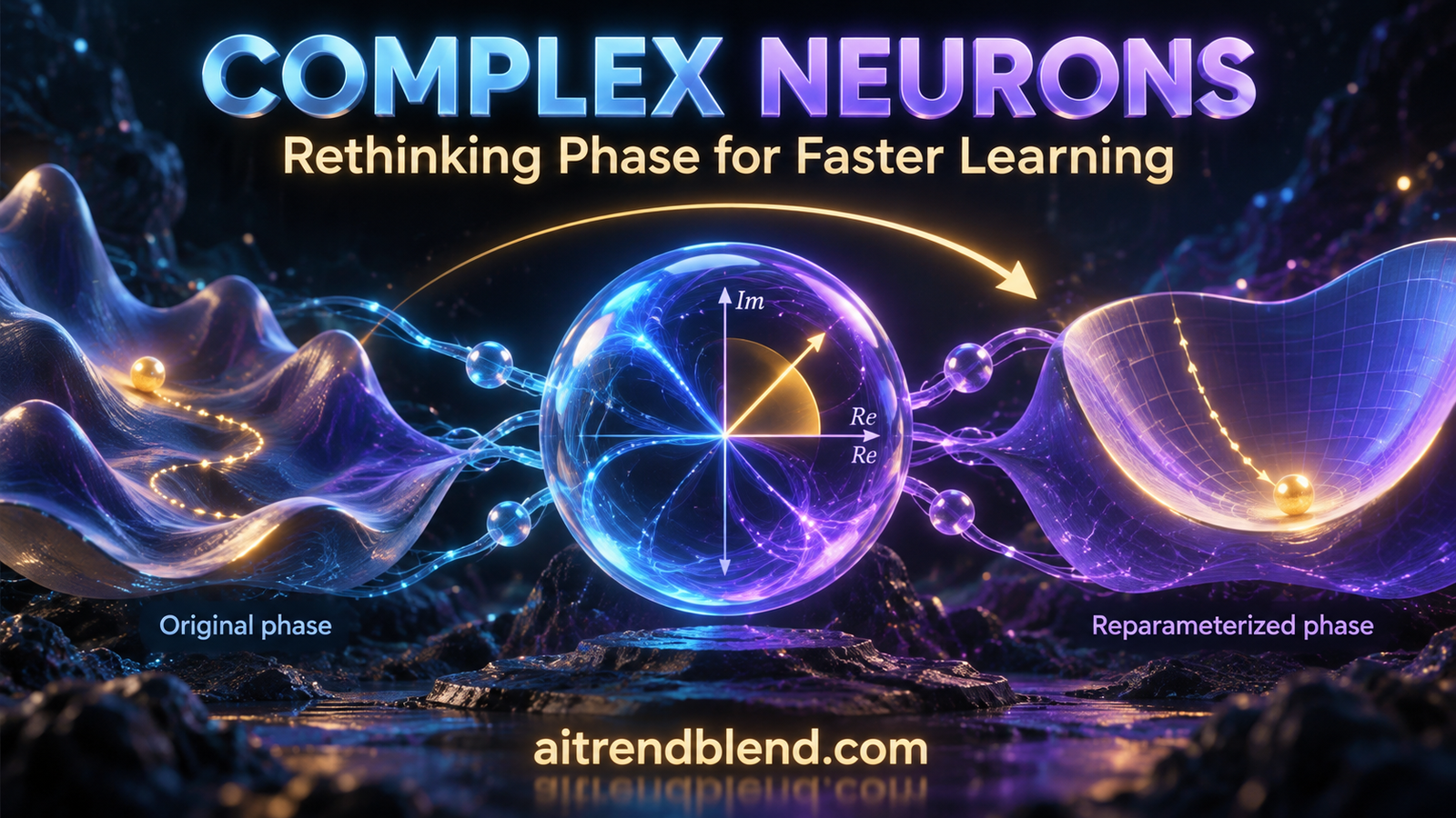
A researcher tests a complex neuron on a target that an ordinary ReLU neuron can learn. The complex model has more flexibility, yet its loss settles into a slow decline. The extra phase parameter can represent useful behavior. In this simpler task, the way it is parameterized also becomes the bottleneck.
- A complex neuron with a learnable angular gate can represent targets that a real ReLU network of fixed finite width cannot reproduce exactly in the studied setting.
- The extra phase freedom can slow learning when the target is an ordinary real neuron.
- The proposed phase reparameterization changes a locally cubic loss dependence into a quadratic one.
- The resulting linear convergence guarantee is conditional and has constant success probability, rather than a guarantee for every initialization.
- The simulations use finite differences for phase updates because the empirical hard gate objective is locally flat in phase.
- The paper provides learning theory and synthetic simulations, not clinical validation or a benchmark study of complete deep networks.
This article explains published machine learning research. The source mentions MRI reconstruction as background motivation, but does not test a clinical reconstruction system. This is not medical advice, diagnosis or treatment guidance. Consult a qualified health professional about personal medical questions.
Reparameterized Complex Neurons Can Efficiently Learn More is a February 2026 publication in the Journal of Machine Learning Research. Jin-Hui Wu, Shao-Qun Zhang, Yuan Jiang and Zhi-Hua Zhou, affiliated with Nanjing University, examine when a complex neuron’s extra capacity helps and when it costs optimization time.
The result belongs in our Optimization & Learning Theory collection. Its practical value is an unusually concrete explanation of an optimization problem. A model can have the right representational capacity and still learn slowly because its parameter coordinates flatten the loss near the desired solution.
The authors extend their earlier NeurIPS study from 2023. The newer contribution is a family of phase reparameterizations, accompanying convergence analysis and simulations. The article below focuses on what changes in the loss geometry, what the learning rates mean and how to implement the hard gate without silently replacing the analyzed model.
More expressive does not automatically mean easier to train
A real neuron takes a weighted sum of real inputs and applies an activation. A complex neuron combines real and imaginary components, allowing its activation to respond to the argument of the complex output. That angular information can distinguish signals that magnitude alone does not explain.
The paper’s introduction points to radar, acoustics and MRI reconstruction as examples where phase information can matter. These are motivations drawn from cited earlier work. They are not applications evaluated by this paper, whose experiments use synthetic targets generated by neurons.
There are at least two separate questions. Can a model represent the target function? Can a particular optimization procedure learn that function efficiently? A positive approximation statement answers the first question, but not the second. The gap is the starting point of the analysis.
Our article about ReLU bases and approximation theory addresses a related distinction from the representation side. Here, the authors follow gradient descent itself, including the speed at which weights and the phase approach their target values.
The conclusion is more specific than a recommendation to replace real arithmetic everywhere. The studied complex activation has an advantage on particular phase sensitive targets. On a real target, an unnecessary phase coordinate can introduce slower convergence. The reparameterization is designed to address that cost.
The activation is an angular gate with a real output
The model uses the real part of a symmetrical version of zReLU. It returns the real component of a complex number when its argument lies inside a sector centered on the positive real axis, and returns zero outside that sector. A phase parameter sets the half width of the active sector.
Equation 1. The symmetrical zReLU output used in Sections 3 and 6.
At a phase of half pi, the active sector becomes the right half plane. Taking its real part then matches an ordinary ReLU response. At zero phase, the active sector has no angular width and the neuron is degenerate under the continuous Gaussian input distribution.
Nondegenerate targets sit strictly between these endpoints and have a nonzero weight vector. That qualification prevents the representation result from being misread as a separation between two models that already coincide at an endpoint.
The output under study is real even though the intermediate weighted input is complex. This is not a complete deep network with arbitrary complex activations or a complex output loss. The model deliberately strips away those complications to expose the learning mechanism.
The input is a real vector with an even number of coordinates, folded into a complex vector. The paper uses a conjugated input in the complex inner product. Keeping that conjugation is important because it makes the real component agree with the ordinary real inner product under the chosen folding convention.
Equation 2. Folded inputs and the complex neuron. The reference code preserves the conjugation rather than using an unconjugated complex product.
The theorem studies population squared loss
The learner tries to match a target neuron on standard Gaussian inputs. Its objective is one half of the expected squared difference between learner and target outputs. Weights and, for a complex learner, the phase are the adjustable parameters.
Equation 3. The objective in Equation 1 of the source. A real target can be represented by the endpoint phase.
The distinction between expected and empirical loss will become crucial later. The theorems analyze an expectation over the Gaussian distribution. A training set of fixed samples instead gives a finite average whose phase dependence has a different local structure.
Most central guarantees assume one complex input dimension, which corresponds to two real coordinates, and omit biases. That lets the authors calculate the expected loss by integrating over angular sectors. It also gives the analysis a sharply defined scope.
The basic complex learner uses projected gradient descent to keep its phase inside the allowed interval. The real learner has no phase parameter. The reparameterized learner replaces phase with another coordinate whose mapping keeps the activation within its valid range.
What complex neurons can learn in the analyzed setting
Theorem 1 concerns a complex learner matching a real target. Under the specified Gaussian weight initialization, uniform phase initialization and a sufficiently small constant step, the paper obtains a loss bound of order the inverse cube of the iteration count, with a success probability lower bound of one in thirty two.
The success qualification is not cosmetic. Some initializations place the learner in an unfavorable angular configuration. The weight can move toward zero while the phase shrinks, producing a stationary failure rather than learning the desired function. A convergence statement therefore needs to specify which initialization event it covers.
Theorem 2 concerns a complex learner matching a complex target. The target phase is restricted to the interval from seven twentieths of pi to two fifths of pi. With a specified decreasing step schedule, the loss has an inverse iteration upper rate and a stated constant probability bound.
Those details narrow the broad summary that a complex neuron learns another complex neuron. The displayed theorem covers a particular target phase interval, an input distribution and a schedule. It should not be described as a uniform guarantee for every activation, phase and dataset.
The authors discuss amplifying success through independent initializations. That introduces extra training and model selection. It is useful as a conceptual response to a constant probability result, but it should not be mistaken for a guarantee that a single random run succeeds with high confidence.
Why the real network lower bound needs careful wording
Theorem 4 compares a nondegenerate complex target with a real network having one hidden ReLU layer and a fixed finite number of neurons. It gives a strictly positive lower bound on expected squared loss, regardless of the choice of the real network’s parameters.
Equation 4. The representation lower bound in Theorem 4. Here (n) denotes hidden width, not sample size.
The lower bound makes an optimization failure unavoidable for exact recovery in that fixed architecture. If the function class cannot achieve zero population loss, a better training algorithm cannot remove the gap. The argument is therefore stronger than a statement about one unlucky training trajectory.
It is also narrower than saying that real neural networks can never approximate complex targets. The bound decreases as the real hidden width grows. The result rules out exact recovery with fixed finite width under the stated setting, not arbitrarily accurate approximation across a sequence of increasing widths.
Biases, depth and alternative activations must be considered separately. The authors believe their insights can extend, but the theorem does not establish an impossibility result for every real network architecture. General universal approximation claims are not contradicted by a positive error floor for a particular fixed class.
This is another reason to keep representation separate from optimization. Our related discussion of pruning and generalization studies how changing the available model structure can change learning behavior. The present lower bound concerns an entirely different target and architecture comparison.
The extra phase can become a slow coordinate
When the target is an ordinary real neuron, its effective target phase is half pi. A complex learner must adjust both its weight and its phase to reproduce that target. Close to the solution, the phase gradient can become much smaller than the phase error.
The authors describe a late convergence regime in which the loss behaves approximately like the cube of the deviation from the target phase. Its derivative with respect to phase behaves like the square of that deviation. Small errors then produce very small updates.
Equation 5. The local behavior motivating Section 6, in the appropriate small angle regime.
Theorem 6 supplies a lower rate result for learning a real target with the original complex parameterization under its local weight condition. Combined with the earlier upper analysis, it identifies a genuine slow phase effect in the examined regime. The slowdown is not merely a loose upper estimate that could hide exponential learning.
The real learner, by comparison, has a cited linear convergence guarantee for learning a real neuron under the assumptions discussed in Lemma 5. Here linear convergence means geometric or exponential decay of error with the iteration count. It does not mean the graph of error falls along a straight line.
More flexibility therefore carries a conditional price. The complex model can represent both kinds of target, but it can spend many late updates adjusting a phase coordinate that the real learner does not need.
An extra parameter can enlarge the function class while making the optimizer’s local job harder. The useful intervention is to examine the coordinate’s loss geometry, rather than assuming capacity alone guarantees efficient learning.
The two thirds power changes the local geometry
The proposed mapping replaces phase with an unconstrained coordinate. A bounded function of that coordinate determines how far the actual phase lies below its upper endpoint. The exponent is chosen to counter the cubic loss behavior.
Equation 6. The real interpretation of the fractional power in Equation 3 of the source. The absolute value makes the expression explicit for either sign of (g).
Substituting this phase deviation into the cubic local loss yields the square of the bounded mapping. Near zero, that mapping is approximately linear in the new coordinate. The loss therefore becomes locally quadratic in the coordinate used by gradient descent.
Equation 7. The approximation in Equation 5 of the source, valid in the analyzed local regime.
The function class is retained through a different route to the phase, while the gradient dynamics change. This is not equivalent to changing the target or replacing the angular gate with a smooth gate. It is a change in the coordinates of the optimization problem.
There is a qualification around endpoints. A function whose range approaches the boundary of the permitted interval only in a limit does not reach every phase at a finite coordinate. The relevant nondegenerate interior phases can still be represented, but exact range statements deserve care.
The source lists sine, hyperbolic tangent and arctangent as possible mappings. The printed range requirement and these examples are not interchangeable without adjustment. Unscaled arctangent is not bounded by one, while hyperbolic tangent approaches rather than attains its extreme values. An implementation should normalize or select its mapping deliberately and check the theorem’s additional conditions.
The listing uses a scaled hyperbolic tangent with local slope one twelfth. It retains interior phases and the real target endpoint at zero coordinate. It treats the degenerate zero phase as a limiting endpoint. That is a disclosed numerical choice, not a claim that the listing validates every abstract range condition.
What the new convergence theorems say
Theorem 7 gives linear convergence for a reparameterized complex learner matching a real target. It assumes the principal input setting, Gaussian initialization of the new coordinate, an appropriate step and a bounded local slope of the mapping.
The slope condition helps preserve the relation between weight alignment and phase movement. Reparameterizing the phase changes its speed, but the argument must keep the trajectory in a region where the favorable quadratic description applies. Faster phase updates are not automatically better if they destroy that region.
The guarantee again has a constant probability lower bound that depends on mapping parameters. The theorem does not say every Gaussian initialization succeeds, and the constants need not match the real learner’s constants. Equal convergence order is different from equal wall clock performance.
Theorem 8 treats a complex target in the same restricted phase interval discussed earlier. It adds monotonicity, Lipschitz and derivative conditions on the mapping and uses a decreasing step schedule. Its inverse iteration convergence order retains the ability to learn the complex target within that setting.
| Learner | Real neuron target | Complex neuron target | Main qualification |
|---|---|---|---|
| Real ReLU neuron or the stated real class | \(O(e^{-c_1t})\) | Positive loss floor for the fixed finite width class | Lemma 5 and Theorem 4 have their respective assumptions |
| Original complex neuron | \(O(t^{-3})\), with a matching lower rate in the discussed local regime | \(O(t^{-1})\) | Specified initialization events, phase range and step conditions |
| Reparameterized complex neuron | \(O(e^{-c_2t})\) | \(O(t^{-1})\) | Additional mapping conditions and constant success probability |
This is a comparison of theorem statements. It is not a benchmark table of accuracy, throughput or GPU memory. The constants and qualifying events differ across the entries, so the table should be read with the surrounding assumptions.
The empirical phase gradient is the implementation trap
For a fixed finite training set and fixed weights, changing phase slightly may leave every sample on the same side of the angular gate. All outputs remain unchanged. Empirical loss is then locally constant in phase until a sample crosses the boundary.
Ordinary autodifferentiation through a Boolean gate does not supply the boundary contribution that appears after integrating over a continuous input distribution. A naive implementation can therefore report zero phase gradients even though the population objective has meaningful phase dynamics.
The authors address this in Appendix H using a difference quotient. They evaluate the empirical loss at perturbed parameter values to approximate the phase gradient used for training. They choose a perturbation width of 0.1 and switch to a one sided difference near a phase domain boundary.
Equation 8. The central difference described in Appendix H, with the appropriate boundary alternative when needed.
The parameter being perturbed must also be identified. A direct complex learner optimizes phase, while the reparameterized learner optimizes the new coordinate. Taking finite differences in phase and then updating the new coordinate without the appropriate relationship changes the intended algorithm.
Our code differentiates the coordinate actually used by each learner. It keeps the hard activation and uses ordinary weight gradients within the currently selected gates. Its separate population mode uses the exact Gaussian cross moment formula for the two dimensional setting, where the integrated loss can be differentiated directly.
The difference quotient is an estimator with a selected scale. It is not an exact finite sample derivative and not a proof that the empirical training trajectory follows the population theorem. That gap is one of the useful lessons of this study, rather than an implementation detail to hide.
Keep the population and empirical objectives separate. Hard angular gates can have meaningful gradients after expectation but zero local phase gradients on a fixed sample. The simulation’s finite difference step is part of the method.
What the synthetic experiments establish
Appendix H specifies training and test sets generated by a randomly initialized target neuron. A real learner, an original complex learner and a reparameterized complex learner are then trained using empirical mean square loss.
| Item | Reported setting |
|---|---|
| Training set | 7,000 synthetic examples |
| Test set | 3,000 synthetic examples |
| Training duration | 100 epochs |
| Learning rate | 0.1 |
| Phase difference width | 0.1 |
| Primary figure setting | One complex dimension and no bias |
| Additional figure setting | Five complex dimensions with bias terms |
Figure 3 shows the complex learners approaching low test errors on a complex target, while the real learner levels off above zero in the displayed runs. Figure 5 shows the reparameterized complex learner behaving much closer to the real learner when the target is real, with the original complex learner decreasing more slowly.
The additional setting broadens the empirical illustration beyond the main theorem’s input dimension and bias restriction. It does not extend the proof to that setting. A simulation curve can support a hypothesis without establishing its theorem conditions.
The paper reports using several random initializations to find trajectories consistent with the theoretical behavior. Appendix H does not provide a numerical restart count or a complete distribution of success and failure outcomes. The displayed curves therefore should not be relabelled as seed averaged performance or a measured probability of success.
The figures also do not provide a numerical table of final losses with confidence intervals. This article describes their visible ordering without inventing precise endpoint values. There is no reported clinical dataset, acoustic benchmark or radar classification accuracy behind those curves.
“neurons cannot always learn a target neuron”Wu and colleagues, Appendix H, discussing simulation outcomes
Clinical translation gap
MRI reconstruction is background motivation, not a clinical experiment in this study. The 7,000 training examples and 3,000 test examples are synthetic neuron generated inputs. They are not patient counts, MRI scans or independent hospital cases.
No patient cohort, diagnostic reference standard or clinical outcome is evaluated. There is therefore no clinical sample size from which to infer medical performance. The source cannot establish how the proposed phase coordinates affect anatomical fidelity, reconstruction artifacts or clinical interpretation.
Gaussian inputs and neuron generated targets also omit scanner differences, acquisition protocols and population variation. Moving toward MRI would require a separate reconstruction model, appropriate data and evaluation of clinically relevant failure modes. That is a research direction, not an outcome established here.
Our MRI reconstruction article discusses a distinct application study. It provides application context rather than evidence that the single neuron reparameterization in this paper is ready for clinical use.
Limits to preserve when testing the idea
The main analysis is about one learner and one neuron target. Deep networks introduce interactions between layers, multiple gates and different optimization geometry. The paper names learning general functions with deep architectures as a future direction.
The loss is an expected Gaussian objective. Learning from finite samples with high probability remains an open direction discussed in the conclusion. The implementation strategy in Appendix H helps run simulations, but does not settle that statistical problem.
The phase mapping also has delicate numerical behavior. Its fractional power can have a singular derivative at zero, even when a favorable composed population loss has a regular local description. A floating point program needs an explicit convention instead of silently claiming smoothness everywhere.
The reference listing uses a stated convention at exactly zero and an explicit piecewise Gaussian moment formula. It is an educational tool for examining the objective. It does not reproduce the authors’ full experiment suite or prove the asymptotic convergence rates.
For a practical comparison, record all initializations and disclose the restart policy. Separate population loss from test loss, keep the target fixed and track which phase coordinate is updated. If a finite difference scale changes the result, report that sensitivity rather than presenting the chosen curve as a universal property.
Our article on batch size and feature learning makes a related point about training dynamics. Changing the optimization procedure can change the phenomenon being studied. Here, replacing the gate or the phase estimator changes the link to the paper.
A coordinate choice can decide what flexibility costs
The core achievement is a learning comparison that separates capacity from optimization. The complex neuron can retain a useful representational advantage, yet its original phase coordinate can slow learning on a simple real target.
The conceptual shift is to inspect the coordinate’s local loss dependence. A cubic phase deviation encourages vanishing updates. The proposed mapping converts that dependence into a locally quadratic form in the new coordinate, making geometric loss decay possible under the analyzed conditions.
The idea may inform other parameterizations where a redundant or constrained coordinate creates flat local geometry. That is a transferable research intuition. It is not proof that the same fractional power improves every gate, optimizer or deep architecture.
The remaining boundaries are clear. Input dimension, Gaussian data, bias restrictions, success events and step schedules all matter. Simulations broaden the illustration, but leave finite sample guarantees and deeper models unresolved.
Future work should test those extensions while making initialization outcomes and phase estimators visible. Application studies would also need task specific metrics, and any medical application would need separate validation that this theory does not provide.
A more flexible neuron need not pay the same learning price in every coordinate system. The useful question is which coordinates let its optimizer use that flexibility.
Complete PyTorch reference implementation
The listing includes real, original complex and reparameterized learners, the hard zReLU output, population and empirical loss functions, finite difference phase updates, training, evaluation and a smoke test. The population mode uses the Gaussian moment expression from Lemma 10 and supports one complex dimension. The empirical mode supports the stated folding in more dimensions, without biases.
This is editorial code rather than authors’ software. The artificial comparison uses one disclosed seed and does not select a successful restart. It reports half mean square error to match the paper’s theoretical loss convention. It is not a claim to reproduce the plotted experimental normalization or results.
Python syntax was checked. An independent numerical calculation verified the Gaussian cross moment formula against angular quadrature in five cases, including contained, partially overlapping and disjoint sectors. PyTorch was unavailable here, so the included PyTorch smoke test was not executed. Run it before extending the example.
"""Editorial companion to Wu et al., JMLR 27(38), 2026.
Requires PyTorch. Uses real and complex single neurons, no biases.
Population objective: exact d=1 Gaussian moments from Appendix A, Lemma 10.
Finite-sample objective: half MSE, with phase difference quotient from Appendix H.
This is not authors' code and does not reproduce their curves or certify theorems.
"""
import math
from dataclasses import dataclass
import torch
from torch import nn

DTYPE = torch.float64


def phase_map(phi):
    # Signed fractional power in Eq. (3) means |g(phi)|**(2/3) over real phi.
    # Scaled tanh is bounded and has local slope 1/12. Endpoint zero is a limit.
    g = torch.tanh(phi / 12)
    if abs(g.detach().item()) == 0:
        # Explicit numerical convention at the map's singular derivative.
        # Do not use this choice as proof of a derivative for all target losses.
        return phi * 0 + math.pi / 2
    return (math.pi / 2) * (1 - g.abs().pow(2 / 3))


class SingleNeuron(nn.Module):
    def __init__(self, d=1, kind='real', seed=42, initial_w=None):
        super().__init__()
        if kind not in {'real', 'complex', 'reparameterized'} or d < 1:
            raise ValueError('Unknown kind or invalid complex dimension')
        gen = torch.Generator().manual_seed(seed)
        self.d, self.kind = d, kind
        w = torch.randn(2 * d, generator=gen, dtype=DTYPE)
        if initial_w is not None:
            w = torch.as_tensor(initial_w, dtype=DTYPE).clone()
            if w.shape != (2 * d,):
                raise ValueError('initial_w must have shape [2*d]')
        self.w = nn.Parameter(w)
        if kind == 'complex':
            self.phase_parameter = nn.Parameter(torch.rand((), generator=gen, dtype=DTYPE) * math.pi / 2)
        elif kind == 'reparameterized':
            self.phase_parameter = nn.Parameter(torch.randn((), generator=gen, dtype=DTYPE))
        else:
            self.register_parameter('phase_parameter', None)

    def phase(self):
        if self.kind == 'real':
            return self.w.new_tensor(math.pi / 2)
        if self.kind == 'complex':
            return self.phase_parameter
        return phase_map(self.phase_parameter)

    def forward(self, x, phase_override=None):
        if x.ndim != 2 or x.shape[1] != 2 * self.d:
            raise ValueError('Expected x[n,2*d]')
        if self.kind == 'real':
            return (x @ self.w).clamp_min(0)
        psi = self.phase() if phase_override is None else phase_override
        # w_C^T conjugate(x_C): real part equals the real-vector inner product.
        xc = torch.complex(x[:, :self.d], x[:, self.d:])
        wc = torch.complex(self.w[:self.d], self.w[self.d:])
        z = (wc[None, :] * xc.conj()).sum(dim=1)
        gate = z.angle().abs() <= psi
        return z.real * gate.to(x.dtype)


def gaussian_cross_moment(w, v, psi_w, psi_v):
    """Lemma 10, d=1, E[sigma_w(X) sigma_v(X)], X~N(0,I_2)."""
    if w.shape != (2,) or v.shape != (2,):
        raise ValueError('Exact moment only supports d=1')
    nw, nv = w.norm(), v.norm()
    if nw.detach().item() < 1e-14 or nv.detach().item() < 1e-14:
        return (w.sum() + v.sum() + psi_w + psi_v) * 0
    aw, av = torch.atan2(w[1], w[0]), torch.atan2(v[1], v[0])
    theta = torch.atan2(torch.sin(aw-av), torch.cos(aw-av)).abs()
    pmin = torch.minimum(psi_w, psi_v)
    factor = nw * nv / (4 * math.pi)
    contained = 2 * torch.cos(theta) * (2 * pmin + torch.sin(2 * pmin))
    partial = (2 * (psi_w + psi_v - theta) * torch.cos(theta)
               - torch.sin(theta - 2 * psi_v) - torch.sin(theta - 2 * psi_w))
    inside = torch.where(theta <= (psi_v-psi_w).abs(), contained, partial)
    return factor * torch.where(theta <= psi_w + psi_v, inside, inside * 0)


def population_loss(model, target):
    if model.d != 1 or target.d != 1:
        raise ValueError('Population formula only supports d=1')
    p, q = model.phase(), target.phase().detach()
    v = target.w.detach()
    return (0.5 * gaussian_cross_moment(model.w, model.w, p, p)
            - gaussian_cross_moment(model.w, v, p, q)
            + 0.5 * gaussian_cross_moment(v, v, q, q))


def sample_loss(model, x, y):
    return 0.5 * (model(x) - y).square().mean()


@torch.no_grad()
def phase_difference_quotient(model, x, y, h=0.1):
    """Differentiate the parameter actually optimized, psi or phi.
    Direct psi uses one-sided differences near domain ends as in Appendix H.
    Reparameterized phi has no projection or phase-domain boundary.
    """
    p = model.phase_parameter
    center = p.item()
    low, high = center - h, center + h
    if model.kind == 'complex':
        if low < 0:
            low = center
        if high > math.pi / 2:
            high = center
    try:
        p.fill_(low)
        left = sample_loss(model, x, y)
        p.fill_(high)
        right = sample_loss(model, x, y)
    finally:
        p.fill_(center)
    return (right - left) / (high - low)


@dataclass
class History:
    loss: list
    phase: list


def train(model, target, steps=100, eta=0.1, objective='sample', x=None, h=0.1):
    if steps < 1 or eta <= 0 or h <= 0:
        raise ValueError('Positive steps, step size and difference width required')
    if objective not in {'sample', 'population'}:
        raise ValueError('Unknown objective')
    if objective == 'sample':
        if x is None:
            raise ValueError('Finite-sample training requires x')
        with torch.no_grad():
            y = target(x)
    history = History([], [])
    for _ in range(steps):
        model.zero_grad(set_to_none=True)
        loss = population_loss(model, target) if objective == 'population' else sample_loss(model, x, y)
        # Hard gates yield no phase derivative through sample-loss autodiff.
        phase_grad = None
        if objective == 'sample' and model.phase_parameter is not None:
            phase_grad = phase_difference_quotient(model, x, y, h)
        loss.backward()
        if objective == 'population' and model.phase_parameter is not None:
            phase_grad = model.phase_parameter.grad.detach().clone()
        history.loss.append(loss.detach().item())
        history.phase.append(model.phase().detach().item())
        with torch.no_grad():
            model.w.sub_(eta * model.w.grad)
            if phase_grad is not None:
                model.phase_parameter.sub_(eta * phase_grad)
                if model.kind == 'complex':
                    model.phase_parameter.clamp_(0, math.pi / 2)
    return history


@torch.no_grad()
def evaluate(model, target, x):
    y = target(x)
    result = {'test_half_mse': sample_loss(model, x, y).item(),
              'phase': model.phase().item()}
    if model.d == 1:
        result['gaussian_population_half_mse'] = population_loss(model, target).item()
    return result


def gaussian_data(n, d, seed):
    return torch.randn(n, 2*d, generator=torch.Generator().manual_seed(seed), dtype=DTYPE)


def smoke_test():
    target = SingleNeuron(kind='real', initial_w=[1., 0.])
    for kind in ['real', 'complex', 'reparameterized']:
        model = SingleNeuron(kind=kind, seed=3, initial_w=[0.9, 0.05])
        if kind == 'complex':
            with torch.no_grad(): model.phase_parameter.fill_(1.2)
        if kind == 'reparameterized':
            with torch.no_grad(): model.phase_parameter.fill_(0.2)
        assert torch.isfinite(population_loss(model, target))
        history = train(model, target, steps=12, eta=0.05, objective='population')
        assert all(math.isfinite(v) for v in history.loss)
        assert history.loss[-1] < history.loss[0]
    # Endpoint activation equals ordinary ReLU, and conjugation has correct sign.
    c = SingleNeuron(kind='complex', initial_w=[1., 2.])
    points = torch.tensor([[1., 1.], [-1., 1.], [0., -1.]], dtype=DTYPE)
    with torch.no_grad(): c.phase_parameter.fill_(math.pi / 2)
    assert torch.allclose(c(points), (points @ c.w).clamp_min(0))
    # Exercise empirical phase updates separately from population derivatives.
    x = gaussian_data(256, 1, 11)
    sample_model = SingleNeuron(kind='complex', seed=5, initial_w=[0.9, 0.05])
    with torch.no_grad(): sample_model.phase_parameter.fill_(1.1)
    grad = phase_difference_quotient(sample_model, x, target(x).detach())
    assert torch.isfinite(grad)
    train(sample_model, target, steps=3, eta=0.05, x=x)
    assert torch.isfinite(sample_model.w).all()
    print('Smoke checks passed; no theorem or rate was certified.')


def artificial_comparison():
    """One disclosed seed, not best-of-restarts or a reproduction of Figure 5."""
    target = SingleNeuron(kind='real', seed=14, initial_w=[1., 0.])
    train_x, test_x = gaussian_data(7000, 1, 20), gaussian_data(3000, 1, 21)
    for kind in ['real', 'complex', 'reparameterized']:
        model = SingleNeuron(kind=kind, seed=22)
        train(model, target, steps=100, eta=0.1, x=train_x, h=0.1)
        print(kind, evaluate(model, target, test_x))
    # For a complex teacher, choose a nondegenerate phase and repeat training.
    complex_target = SingleNeuron(kind='complex', initial_w=[1., 0.])
    with torch.no_grad(): complex_target.phase_parameter.fill_(3*math.pi/8)
    student = SingleNeuron(kind='reparameterized', seed=23)
    train(student, complex_target, steps=100, eta=0.1, x=train_x)
    print('Complex target demonstration:', evaluate(student, complex_target, test_x))


if __name__ == '__main__':
    smoke_test()
    artificial_comparison()
Frequently asked questions
Are complex neurons always better than real neurons?
No. The result concerns particular neuron classes, Gaussian objectives and conditional learning guarantees. The original complex learner can converge more slowly on a real target.
What does linear convergence mean here?
It means geometric or exponential decay of the loss with the iteration count under the stated conditions. It does not mean error decreases by a fixed amount each iteration.
Can a real network never approximate a complex neuron?
Theorem 4 gives a positive population loss floor for the stated real ReLU class with fixed finite width. It does not forbid increasingly accurate approximation when width grows or establish the same result for every architecture.
Why does the code use finite differences for phase?
The empirical hard gate objective is locally constant in phase between sample boundary crossings. Appendix H uses a difference quotient to estimate the phase update rather than relying on the local derivative of that fixed sample loss.
Does this paper validate MRI reconstruction or medical diagnosis?
No. MRI reconstruction is cited as background motivation. The experiments use synthetic neuron generated inputs and provide no clinical cohort, reconstruction validation or diagnostic evidence.
Has the reference code reproduced the published curves?
No. It is an editorial implementation with disclosed mapping and numerical choices. Syntax and an independent Gaussian moment calculation were checked. The PyTorch smoke test was not run here, and the code does not claim to reproduce the authors’ curves.
Inspect the proof and the reference implementation
The paper provides the convergence conditions, lower bound argument and synthetic simulation details. The downloadable code is the educational listing included here.
Read the JMLR paperDownload reference codeWu, J. H., Zhang, S. Q., Jiang, Y., and Zhou, Z. H. (2026). Reparameterized Complex Valued Neurons Can Efficiently Learn More than Real Valued Neurons via Gradient Descent. Journal of Machine Learning Research, 27(38), pages 1 to 51. Title punctuation simplified. Official publication record.
This analysis is based on the published paper and an independent evaluation of its claims.