
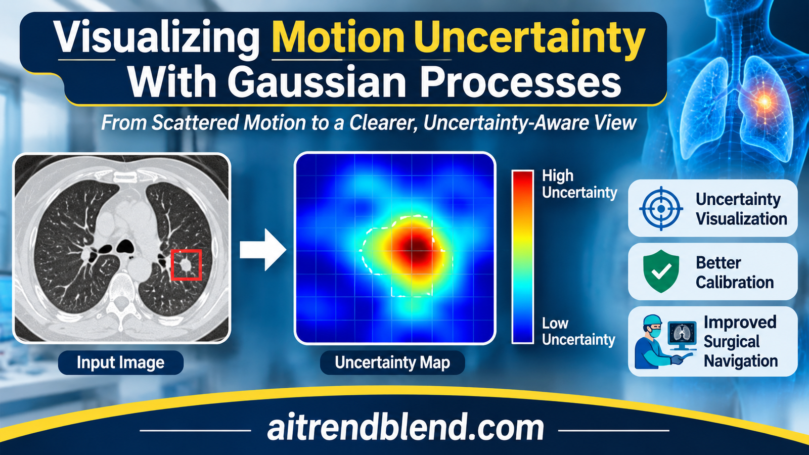
A radiologist is about to take a needle biopsy from a small breast lesion. The lesion was marked on an MRI acquired before the procedure, with the patient in a different position and the breast under no pressure. Now the breast is compressed, the needle is pressing on the skin, and the navigation screen shows where the software thinks the lesion has moved. It shows one answer, drawn with the same crisp edges whether the estimate is excellent or a rough guess.
That last detail is the subject of a paper by Bojan Kocev, Horst Karl Hahn, William M. Wells, Lars Linsen and Ron Kikinis, working across Constructor University Bremen, Fraunhofer MEVIS, the University of Münster, the University of Bremen and Harvard Medical School with Brigham and Women’s Hospital. Their method takes a Gaussian process that estimates soft tissue motion with error bars, and turns those error bars into pictures a clinician could read at a glance. The clever part is a grid that blurs wherever the motion is uncertain. The open question is whether anyone at the bedside reads it the way the authors intend.
Key points
- The method propagates the uncertainty of a Gaussian process motion model into three pictures, a deformed image with a blurred grid laid over it, probability contours for where a region such as a tumor ended up, and a probability map for where a single point moved.
- Blur is applied to an artificial grid, never to the patient image, so the anatomy stays sharp while the grid shows how far to trust each part of it.
- The main numerical test is one inhale and exhale lung CT pair from the DIR-Lab COPDGene archive. Leaving out each of 300 expert landmarks in turn, the model’s mean 3D error was 1.782 mm and its uncertainty was close to calibrated.
- Our arithmetic on the reported numbers points to mild overconfidence in the tails. The average squared Mahalanobis distance of 3.499 sits about 3.5 standard errors above the ideal of 3, even though a Kolmogorov-Smirnov test did not flag a difference.
- The predicted uncertainty ranks errors only moderately, with a Spearman correlation of 0.391 against the 3D error. It flags the worst landmarks but is not a precise per point warning.
- No clinician or surgeon evaluated the visualizations. For a paper whose product is a picture meant to change decisions, that is the largest gap.
Medical disclaimer. This article explains published research on image guided intervention software. It is not medical advice, diagnosis or treatment, and it does not evaluate any approved clinical product. Navigation and registration software used on patients must be validated and supervised by qualified professionals. If you have questions about a procedure, please talk to your care team.
The problem with a confident looking registration
Many procedures are planned on images taken days or hours before the patient arrives in the treatment room. A tumor is outlined on MRI, a needle path is drawn on CT, a radiation beam is shaped around an organ. By the time the plan is used, the anatomy has moved. Lungs inflate and deflate, a breast is compressed, organs shift when a patient lies differently. Software therefore deforms the planning image to match the current state of the body, a step known as deformable registration, and the deformed image guides the clinician.
Every such deformation is an estimate. It rests on sparse or noisy measurements of how tissue moved, on a model of how tissue usually moves, and on interpolation between the two. Some regions are pinned down by many measurements and some are far from any. Yet the deformed image on the screen carries no trace of that difference. A pixel that the software is sure about looks exactly like a pixel it guessed.
Researchers have known for years how to attach error bars to registration. Christian Wachinger, Polina Golland, Martin Reuter and William Wells showed at MICCAI 2014 that Gaussian process interpolation could estimate uncertainty in image registration. Kocev and the same group of coauthors published a Gaussian process model in 2019, uncertainty aware asynchronous scattered motion interpolation, that handles motion samples scattered unevenly in space and time and returns a full posterior distribution over motion. What was missing was a way to show that posterior to a person without drowning them in numbers. That is the gap the new paper, Motion uncertainty visualization based on Gaussian process regression, sets out to fill.
Our earlier article on FlexiMIND and training free deformable registration of CT and MRI covers the registration side of this story, where the goal is the most accurate single answer. This paper asks a different question. Given an answer and its uncertainty, what should the screen look like? More registration, reconstruction and motion work sits in our Medical AI section.
What the visualization literature already knew
The paper leans on a body of visualization research that most medical imaging readers will not have met. Two findings frame the design. Harrower’s 2003 survey of map based uncertainty displays drew two principles from earlier evaluations, that displays integrating value and certainty work better than showing each separately, and that users prefer static displays over ones that toggle between value and certainty. Bonneau and colleagues, in their 2014 overview, listed the visual variables that people naturally read as uncertainty, namely blur, flicker, reduced saturation, sketched outlines and transparency.
Bonneau and colleagues also added a warning that the authors quote honestly. Blurring a visualization does tell viewers that confidence is lower, but it does not by itself lead to better informed decisions. Deitrick’s work in cartography found that showing uncertainty does change the decisions people make, and work by Politi and colleagues suggests that showing patients the uncertainty in the outcome of a medical intervention may improve satisfaction with shared decisions and lower regret. Whether a particular display helps is an empirical question about people, not a property of the algorithm.
Closer to the method itself, Botchen and colleagues blurred streaklines to show uncertainty in time varying 2D flow, and Lodha and colleagues visualized the uncertain position of moving particles with glyphs, transparency and pseudo color. Saad and colleagues built ProbExplorer and related tools for exploring probabilistic medical image segmentations. Kocev’s group borrows from all three, but in an image guided setting where the clinician has seconds, not minutes, to read the screen.
From scattered motion samples to a posterior over deformations
The starting point is the 2019 motion model. Each training sample is a location in space and two time points, paired with how far the tissue at that location moved between them. Samples can arrive at different times and from different places, and each carries its own measurement noise. A Gaussian process, a flexible prior over smooth functions described in detail in the textbook by Carl Edward Rasmussen and Christopher Williams, is conditioned on those samples. The result is not one motion field but a distribution over motion fields, with a mean and a variance at every location.
Gaussian process regression, one scalar output at a time (Eq. 1)
$$ f \mid \mathcal{D} \sim \mathcal{GP}(m_{\mathcal{D}}, k_{\mathcal{D}}) $$ $$ m_{\mathcal{D}}(x) = m(x) + \Sigma(X, x)^{\top} (\Sigma + \sigma_n^2 I)^{-1} (y – \mu) $$ $$ k_{\mathcal{D}}(x, x’) = k(x, x’) – \Sigma(X, x)^{\top} (\Sigma + \sigma_n^2 I)^{-1} \Sigma(X, x’) $$\(X\) holds the training locations, \(y\) the measured displacements, \(\mu\) the prior mean at the training points and \(\Sigma\) their covariance. The 2019 model uses a non constant mean and an anisotropic covariance, and fits one independent GP per displacement axis.
Two modelling choices from the earlier work carry through. The mean of the prior is not constant, because the authors argue that motion samples scattered unevenly in space and time are poorly summarized by their average. The covariance is anisotropic, so motion can vary faster along one direction than another. Each displacement axis gets its own GP, which keeps the mathematics simple and, as we will see, means the uncertainty at each point is an ellipsoid aligned with the image axes. The authors fitted everything with the GPML toolbox in MATLAB.
For the main medical scenario the training data come from simulation. The team built a finite element model of the CIRS triple modality breast biopsy training phantom, a commercial teaching phantom, with 1962 vertices, and pushed on it with a point force at a chosen biopsy insertion point, directed toward the phantom’s centroid. The largest simulated deformation was about 16.19 mm. From this nonlinear but physically plausible motion they drew a small set of randomly scattered samples, added noise whose size varied from sample to sample, and kept the rest as noise free ground truth. The authors point out that the material properties need not match the real phantom exactly, since the test only asks whether the method can recover whatever motion the simulation produced.
How the uncertainty becomes a picture
The expected deformed image
Think about what a distribution over motion fields means for a single voxel of the deformed image. Under the most likely field, one particular source voxel lands there. Under other plausible fields, its neighbors might. The expected deformed image averages over all of them, weighting each nearby source voxel by the probability that it moved to this exact spot.
Expected deformed image (Eqs. 3 and 4)
$$ \bar{\mathbb{B}}_{i,j,k} \approx \sum_{u,v,w} \mathbb{P}^{\,i,j,k}_{u,v,w}\, \mathbb{A}_{\,i+s-u,\; j+s-v,\; k+s-w} $$\(\mathbb{A}\) is the input image and \(\mathbb{P}^{\,i,j,k}_{u,v,w}\) the probability that voxel \((i+s-u, j+s-v, k+s-w)\) moves to voxel \((i, j, k)\), computed from the Gaussian posterior mean and covariance of its displacement. The kernel spans \((2s+1)^3\) voxels and the weights are normalized by their sum at each voxel. The authors tried \(s < 20\) and found \(s = 9\) worked best.
Applied to a patient image, this gives a blurred image, sharper where motion is certain and smeared where it is not. The authors deliberately do not show that blurred patient image to the clinician. Instead they show the maximum a posteriori image, the single most likely deformation, made by pushing every voxel along the posterior mean.
Most likely deformed image by forward mapping (Eq. 5)
$$ \hat{\mathbb{B}}_{(i,j,k) + \bar{\mathbb{U}}(i,j,k)} = \mathbb{A}_{i,j,k} $$\(\bar{\mathbb{U}}\) is the posterior mean displacement in voxel units. Because every source voxel is pushed forward, some target voxels receive nothing and stay empty. The authors keep these holes on purpose, as visible evidence that no tissue was predicted to arrive there.
A window with glazing bars
Here is where it gets interesting. To show uncertainty without degrading the anatomy, the authors run the expected deformation on a different input, an image of a regular 3D grid the same size as the scan. Where motion is certain, the grid lines arrive sharp. Where it is uncertain, they smear, and the direction of the smear follows the direction of the uncertainty. The authors compare the result to looking through a window with glazing bars. The view outside is the most likely anatomy, and the bars themselves carry the doubt.
“we are not blurring the actual data but an artificial grid”
Kocev and colleagues, on why the patient image stays untouched
Two recipes combine the most likely image \(\hat{\mathbb{B}}\) with the blurred grid \(\bar{\mathbb{B}}\). Both use a threshold \(\tau\) that controls how much of the blurred grid is allowed to show.
Alpha blending and masking, each with a threshold (Eqs. 6 to 9)
$$ \mathbb{C}_{i,j,k} = \alpha\, \hat{\mathbb{B}}_{i,j,k} + (1 – \alpha)\, \mathcal{T}(\bar{\mathbb{B}}_{i,j,k}, \tau), \qquad \mathcal{T}(z, t) = \begin{cases} z & z \ge t \\ 0 & \text{otherwise} \end{cases} $$ $$ \mathbb{C}_{i,j,k} = \mathcal{M}\big(\hat{\mathbb{B}}_{i,j,k}, \mathcal{T}(\bar{\mathbb{B}}_{i,j,k}, \tau)\big), \qquad \mathcal{M}(z, z’) = \begin{cases} z’ & z’ > 0 \\ z & \text{otherwise} \end{cases} $$With \(\tau = 0\) the first recipe is plain alpha blending. For the lung CT case the authors scale both images to the range 0 to 1, use \(\alpha = 0.75\), and add a gamma correction to the thresholded grid to raise contrast.
All results are shown as 2D cross sections. The authors considered and rejected volume rendering, because a dense 3D display of both the anatomy and the uncertainty would hide features behind each other, and transparency would blend them in ways a viewer cannot pull apart again.
Where did the tumor go, and where did this point go
The second level of the visualization works on a region of interest such as a tumor. It starts from a probabilistic segmentation of the region in the planning image, where each voxel holds a marginal label probability, the chance that it belongs to the region. A deterministic outline is just the special case of ones and zeros. Running that probability map through the same expected deformation gives approximate label probabilities after deformation, which can be shown in grayscale or as contours at chosen probability levels. On the breast phantom the authors drew contours at 0.01, 0.1, 0.25 and 0.5. The spread between the outer and inner contours is the uncertainty about where the lesion now sits.
The third level shrinks the region to a single voxel, a point of interest such as a tumor centroid. Its deformed probability map, colored and laid over the planning image next to the original point, shows how far and in which direction the point is likely to have gone. On the phantom, both the region contours and the point map stretched further horizontally than vertically, matching the direction in which the grid blurred most.
Key takeaway
One operation, the expected deformation of Eqs. 3 and 4, produces all three displays. Feed it a grid and you get the global uncertainty picture. Feed it a segmentation and you get probability contours for a region. Feed it a single voxel and you get a probability map for a point. The anatomy itself is only ever shown at its most likely position.
The four test scenarios
The paper tests the method on four kinds of data, and only one of them produces numbers that can be checked against an independent reference. The table below sorts them by what kind of evidence each provides.
| Scenario | Motion data | Ground truth | How results were judged |
|---|---|---|---|
| Breast biopsy phantom, MRI | Scattered noisy samples from a finite element simulation, largest deformation about 16.19 mm | Noise free simulation output | Visual inspection of grids, contours and point maps |
| Synthetic 2D field | Analytic Sine-Gordon function, 10, 20 or 50 samples, noise from 0.01 to 0.1 | Exact function | Visual comparison of contours with the true deformed slice |
| Lung CT, inhale to exhale | 300 expert landmarks on DIR-Lab COPDGene case 1 | Each left out landmark in turn | Calibration and accuracy statistics, plus visual inspection |
| Hurricane Isabel simulation | 150 scattered samples of wind driven motion in 5D, with and without added noise | Eye wall at the next hour of the simulation | Visual overlay of predicted and true eye wall |
The phantom and the synthetic field
On the breast phantom the authors compare two deformation estimates, one moderately uncertain and one very uncertain along a single direction. The holes in the most likely image hint at the difference, since the more uncertain estimate leaves more of them, but holes are a weak signal. An image without holes is not necessarily certain. The blurred grid makes the difference obvious, and it blurs more along the horizontal axis, which the authors trace to the axis along which the second deformation was uncertain.
The synthetic test uses the exact solution form of the 2D Sine-Gordon equation, following Gu and Hu, to generate motion with known ground truth. The authors vary the number of samples between 10, 20 and 50 and the noise level between 0.01, 0.025, 0.05 and 0.1, and report that more noise produced visibly wider uncertainty while more samples produced better interpolation. That matches intuition, but the evidence is a grid of twelve small figures judged by eye. One small reproducibility note from our own check. With the printed parameters, the dispersion condition the solution requires holds for the first wave, where 1.21 plus 0 minus 0.21 gives 1, but gives 1.09 for the second and third. The function is still smooth and fully known, so the interpolation test is not affected, but it is not an exact solution of the equation as stated.
The hurricane, a test outside medicine
The most unusual scenario is a weather simulation of Hurricane Isabel from September 2003, produced at the National Center for Atmospheric Research. The data cube is 500 by 500 by 100 points covering about 2139 km by 2004 km by 19.8 km, with 48 hourly time steps. The authors segment the eye wall by thresholding wind speed at 50 km/h, build 150 scattered motion samples from the wind field, and predict where the eye wall will be an hour later. They had to replace the squared exponential covariance with a Matérn covariance, which allows rougher and more local variation, to fit atmospheric motion.
The prediction was not perfect, which the authors expected from 150 samples in a 5D space. The useful observation is that the uncertainty display agreed with the error. The lower part of the eye wall, where the prediction was poor, also showed low probabilities. Adding noise with a standard deviation of 0.2 times the average displacement made the prediction more uncertain, and the display showed that too. It is a sensible demonstration that the machinery is not tied to soft tissue, though it carries no clinical weight.
The lung CT test, where the numbers live
The quantitative core of the paper uses one inspiratory and expiratory breath hold CT pair, case 1 of the DIR-Lab COPDGene reference data described by Richard Castillo and colleagues in 2013. COPDGene is an observational study of chronic obstructive pulmonary disease across 21 United States clinical centers. Case 1 is a volume of 512 by 512 by 121 voxels, each 0.625 by 0.625 by 2.5 mm, with 300 expert landmark pairs. The landmarks move 25.90 mm on average, with a standard deviation of 11.57 mm, and repeated identification by several observers differs by 0.65 mm on average.
The GP is trained on the landmark displacements and then used to deform the inhale CT toward exhale. For this large motion the authors adapt the method in two ways. The most likely image is made by inverse mapping with trilinear interpolation, which avoids holes, and the expected deformation uses a kernel centered on each voxel’s predicted source location, with its size along each axis set from the predicted standard deviation. Region probabilities for the right and left lung, drawn as contours at 0.01, 0.5 and 0.9, show some uncertainty about where the lungs end up, but not much.
Then comes the calibration test, the part of the paper a statistician will care about most. For each of the 300 landmarks, the GP is conditioned on the other 299 and asked to predict the left out one. Each prediction comes with a mean and a variance per axis, so every landmark gives a squared Mahalanobis distance, the squared error measured in units of predicted standard deviations. If the uncertainties are right and the errors Gaussian, those distances follow a chi square distribution with three degrees of freedom, whose mean is 3.
Two ways to score an uncertain prediction
$$ d^2 = \sum_{a \in \{\mathrm{RL}, \mathrm{AP}, \mathrm{SI}\}} \frac{(y_a – \mu_a)^2}{\sigma_a^2} \;\sim\; \chi^2_3 \ \text{if calibrated} $$ $$ \mathrm{NLPD}(y \mid \mu, \sigma^2) = \frac{1}{2} \left[ \frac{(y – \mu)^2}{\sigma^2} + \log \sigma^2 + \log(2\pi) \right] \qquad \text{(Eq. 13)} $$RL, AP and SI are the right to left, front to back and head to foot axes. The negative log predictive density punishes both large standardized errors and needlessly wide uncertainty, so it is minimized only when the mean is accurate and the variance matches the actual error.
| Measure | RL | AP | SI | Overall |
|---|---|---|---|---|
| NLPD, Gaussian process | 1.393 | 1.503 | 1.727 | 1.541 |
| NLPD, constant baseline | 3.086 | 3.824 | 3.685 | 3.532 |
| Spread of the baseline in mm, our arithmetic | 5.30 | 11.08 | 9.64 | n/a |
| Spearman, predicted SD against error | 0.289 | 0.239 | 0.194 | 0.391 in 3D |
| MAE in mm | 0.763 | 0.856 | 1.053 | n/a |
| RMSE in mm | 1.038 | 1.237 | 1.390 | n/a |
| RMSE divided by MAE, our arithmetic | 1.36 | 1.45 | 1.32 | 1.25 if Gaussian |
| Target registration error in 3D, mm | mean 1.782, standard deviation 1.169, maximum 8.158 | n/a | ||
The headline statistics look good. The mean squared Mahalanobis distance was 3.499 against an ideal of 3, a Kolmogorov-Smirnov test against the chi square distribution did not reject it, with a p value of 0.149, and per axis coverage curves, the share of landmarks whose error falls within half to three predicted standard deviations, track the Gaussian ideal closely. All three per axis Spearman correlations between predicted standard deviation and actual error were positive with p below 0.001. The GP’s NLPD was lower than the baseline’s on every axis, an average gain of 1.99 nats per axis, or about 5.97 nats per landmark.
Reading the calibration numbers more closely
The numbers tell a slightly more complicated story than the word calibrated suggests. Under a chi square distribution with three degrees of freedom the variance is 6, so the average of 300 independent values has a standard error of about 0.14. A mean of 3.499 is therefore roughly 3.5 standard errors above 3, by our arithmetic. The leave one out predictions share most of their training data, so the values are not fully independent and the true standard error is somewhat larger, but the direction is clear. On average the GP’s variances are a little too small. Scaling every predicted standard deviation up by about 8 percent would bring the mean to 3.
Why did the Kolmogorov-Smirnov test not object? It compares whole distributions and is most sensitive near the middle, where most values sit. The authors themselves note a slightly heavier right tail, with a few landmarks reaching squared distances near 30, where the ideal distribution has almost no mass. The ratio of root mean square error to mean absolute error points the same way. For Gaussian errors that ratio is about 1.25. Here it is 1.32 to 1.45 per axis, the signature of a few errors much larger than the rest. The largest single error, 8.158 mm, is more than four times the mean. In the paper’s Figure 26 the coverage curves also appear to sit a little under the ideal at the widest intervals.
None of this undermines the main result. The GP is close to calibrated in the bulk, and a few percent of overconfidence is common in practice. It does matter for the clinical story, though, because the tails are where the dangerous cases live. A display that shows a landmark as confidently placed when it is in fact 8 mm off is exactly the failure an uncertainty display exists to prevent.
What the baseline comparison shows, and what it does not
The NLPD comparison sets the GP against a trivial predictor that guesses the average displacement of all landmarks, with the overall spread of the landmarks as its uncertainty. The paper gives its NLPD formula, which lets us back out that spread, about 5.3, 11.1 and 9.6 mm along the three axes. A gain of 1.99 nats per axis means the GP assigns roughly 7 times more probability density to the true displacement than this baseline does. That is a real improvement, but the baseline knows nothing about where a landmark is. Any interpolation method would beat it. A stronger reference, such as a thin plate spline or a GP with a constant mean, would tell readers how much of the calibration comes from the specific modelling choices of the 2019 model.
The Spearman correlation of 0.391 between total predicted uncertainty and 3D error is the honest measure of how useful the uncertainty is for an individual landmark. It is clearly positive. The landmarks with the largest predicted uncertainty, above about 3 mm, include the largest errors. But a moderate rank correlation also means many landmarks with ordinary looking uncertainty carry large errors, and the paper describes the uncertainty, fairly, as a useful but not exact per landmark reliability indicator.
Key takeaway
On 300 lung landmarks the GP’s uncertainty is close to calibrated, about 7 times more informative per axis than a naive guess, and positively linked to error. By our reading of the same numbers, it runs slightly overconfident, mostly because of a handful of large errors, and it ranks individual errors only moderately well.
Why 1.782 mm is not a registration benchmark score
A mean target registration error of 1.782 mm on a COPD lung case can look like a strong registration result. It should not be read as one. In this test the GP is trained on 299 expert landmark correspondences and asked to interpolate the 300th. It never looks at the images to find the motion. Image based registration methods, by contrast, must discover the correspondences themselves from intensities, and the landmarks are held out entirely for evaluation. The two numbers answer different questions. For a sense of scale only, our FlexiMIND article reports an image based method reaching 1.27 mm on the separate DIR-Lab 4DCT cases, a different dataset with smaller motion. The fair comparison for this paper’s TRE is the inter observer error of 0.65 mm, which it exceeds by a factor of about 2.7, and the 2.5 mm slice spacing, which it beats.
Our own toy check of the method
The authors could not share their data, and no code was released, so we wrote a PyTorch reconstruction of every equation and ran it on a version of the synthetic Sine-Gordon test. It uses the paper’s parameters, a 48 by 48 pixel slice with a soft tissue blob and a small lesion, sample counts of 10 to 100 and noise levels of 0.01 and 0.1. Unlike the paper, we scored the results numerically, on 300 random pixels to mirror the 300 landmarks, and averaged three random seeds. We also tried two ways of implementing the non constant mean, because the paper does not spell out its exact form.
| Mean | Noise | Samples | MAE | Predicted SD | Mean d² | Coverage at 2 SD | NLPD | Band |
|---|---|---|---|---|---|---|---|---|
| Integrated | 0.01 | 10 | 0.60 | 0.24 | 20.37 | 0.428 | 4.48 | 9 |
| Integrated | 0.01 | 20 | 0.26 | 0.18 | 6.30 | 0.692 | 0.64 | 1 |
| Integrated | 0.01 | 50 | 0.11 | 0.12 | 3.25 | 0.869 | −0.47 | 0 |
| Integrated | 0.01 | 100 | 0.07 | 0.10 | 1.82 | 0.963 | −0.99 | 0 |
| Integrated | 0.1 | 10 | 2.06 | 1.06 | 14.01 | 0.681 | 4.44 | 66 |
| Integrated | 0.1 | 20 | 1.00 | 0.98 | 3.53 | 0.888 | 1.68 | 47 |
| Integrated | 0.1 | 50 | 0.57 | 0.57 | 3.70 | 0.874 | 1.26 | 28 |
| Integrated | 0.1 | 100 | 0.38 | 0.43 | 3.06 | 0.885 | 0.81 | 17 |
| Point estimate | 0.01 | 10 | 0.62 | 0.14 | 130.52 | 0.221 | 31.37 | 2 |
| Point estimate | 0.01 | 20 | 0.28 | 0.14 | 19.25 | 0.485 | 3.58 | 1 |
| Point estimate | 0.01 | 50 | 0.12 | 0.10 | 5.62 | 0.799 | −0.08 | 0 |
| Point estimate | 0.01 | 100 | 0.08 | 0.09 | 2.85 | 0.903 | −0.84 | 0 |
| Point estimate | 0.1 | 10 | 3.07 | 0.40 | 835.30 | 0.237 | 208.70 | 23 |
| Point estimate | 0.1 | 20 | 1.57 | 0.79 | 22.24 | 0.512 | 6.08 | 48 |
| Point estimate | 0.1 | 50 | 0.67 | 0.29 | 15.70 | 0.481 | 3.58 | 11 |
| Point estimate | 0.1 | 100 | 0.51 | 0.28 | 13.50 | 0.603 | 2.98 | 6 |
The broad pattern the paper describes by eye shows up in the numbers. With the integrated mean and low noise, the average error fell from 0.60 to 0.07 pixels as the samples grew from 10 to 100, and the predicted standard deviation fell with it. With ten times more noise, the predicted uncertainty was several times larger, and the band of pixels where the lesion’s probability was neither near 0 nor near 1 shrank from 66 to 17 pixels as data were added. More noise widened the uncertainty and more data narrowed it, as in the paper’s Figures 12 to 15.
Calibration was another matter. With only 10 samples the GP was badly overconfident, with mean squared Mahalanobis distances of 20.37 and 14.01 where 2 is ideal, and its NLPD of about 4.5 was worse than the constant baseline’s 1.82. By a proper scoring rule, an overconfident GP fitted to very little data did worse than no model at all. Calibration became good only at 50 to 100 samples, which is reassuring for the paper’s lung test with 299 training landmarks and a warning for any intraoperative setting where motion samples are sparse.
The form of the non constant mean mattered more than we expected. Fitting a linear trend as a point estimate, the obvious implementation, left the GP far more overconfident, with a mean squared distance of 130.52 at 10 samples and still 13.50 at 100 noisy ones, because the uncertainty in the fitted trend never reaches the predictive variance. Integrating the trend out, as described in Section 2.7 of the Rasmussen and Williams textbook, removed most of the problem. The paper does not say which form its mean takes, so anyone reimplementing the method should check their calibration rather than assume it.
These are toy numbers on a 48 by 48 slice with our own modelling choices. They say nothing about the paper’s results and are meant only to show how the pieces behave.
Clinical translation gap
The intended setting is clear from the paper’s funding and examples. The German Research Foundation supported it through a creative unit called Intra Operative Information, What Surgeons Need, When They Need It, and the authors write that the type of display in their region of interest figures would be particularly useful for biopsy specialists navigating in deforming tissue. The distance from this paper to that setting is long, and most of it is about people rather than mathematics.
First, the method has not met its users. Nobody tested whether radiologists or surgeons read a blurred grid as intended, whether it slows them down, whether it makes them more cautious in the right places, or whether it simply adds clutter. The authors’ own sources warn that blur signals lower confidence without guaranteeing better decisions. The conclusion names a user evaluation with surgeons as future work, which is the right next step and also the one that decides whether the idea succeeds.
Second, the motion data are not intraoperative. The breast results use a simulated phantom, the synthetic results an analytic function, and the lung results expert landmarks placed afterwards on high quality breath hold CT. During a real biopsy, motion measurements would come from tracked instruments, surface sensors or fast imaging, with their own delays and failure modes. How the 2019 GP behaves with that kind of input is untested here.
Third, timing is not reported. With the fixed kernel at \(s = 9\), every output voxel looks at 6,859 neighbors. Applied to a volume the size of COPD case 1, that would be about \(2.2 \times 10^{11}\) likelihood evaluations by our arithmetic, for one display. The authors note the computation is highly parallel and propose a GPU version, and they identify inverting the covariance matrix as the bottleneck for larger training sets, with sparse and low rank approximations as remedies. Until then, the method suits planning and review better than live guidance.
Fourth, the uncertainty covers motion only. The examples treat the region segmentation in the planning image as certain, although the method can accept a probabilistic one, and the uncertainty of the segmentation model itself, the imaging, and the tracking of the instrument would all add to the total that a clinician actually faces.
Regulatory and safety note, our reading
Navigation software that tells a clinician where a lesion has moved would be regulated as a medical device in most jurisdictions, and an uncertainty display would become part of its claims and its instructions for use. That raises questions this paper does not address. What should a user do when the grid blurs over the target? How are users trained to read it? What happens when the display looks confident but the estimate is wrong, as in the tail cases above? Any clinical version would need calibration checks on local data, human factors testing with the intended users, and clear escalation rules before a blurred region could change a procedure.
Limitations, sample size and bias
- One CT pair carries all the statistics. Every calibration and accuracy number comes from case 1 of the DIR-Lab COPDGene set, one patient with 300 landmarks. The other nine cases in that archive were not used, so nothing is known about variation between patients.
- Interpolation, not registration. The lung test interpolates between expert landmarks rather than registering images, so its 1.782 mm error is not comparable with image registration results on the same archive.
- Visual judgment elsewhere. The phantom, synthetic and hurricane results are assessed by looking at figures. There are no reader studies, no error statistics for the synthetic grid of experiments and no comparison with other uncertainty displays.
- Simulated soft tissue. The breast results rest on a finite element simulation of a training phantom with a largest deformation of about 16.19 mm, not on patient data or measured phantom motion.
- Axis aligned uncertainty. Each displacement axis has its own GP, so the predicted covariance is diagonal. Real tissue motion, such as lungs sliding along the chest wall, is correlated across axes, and a diagonal model cannot show a tilted uncertainty ellipse.
- Tuning by eye. The kernel size \(s = 9\) is described as the most optimal of the values tried, without the criterion behind that choice. The thresholds, opacity and gamma values that shape every figure are set interactively.
- Normalization hides arrival. By our reading of Eqs. 3 and 4, the weights are normalized at every voxel, so the expected image shows what would arrive if anything arrives, not how likely it is that anything arrives at all. The holes in the most likely image partly fill that role. Our code returns the unnormalized weight sum as an optional extra map.
- No data or code. The authors state they do not have permission to share data. The lung case is available from DIR-Lab on request, but the breast simulation and the exact GP settings are not, which limits independent replication.
What practitioners can take from this
For anyone building registration or motion tracking tools, the most transferable idea is the separation between the anatomy and the uncertainty. Showing the most likely image untouched and putting the doubt on an overlay respects what clinicians are used to reading, and it can be added to any method that outputs a mean and a variance per voxel, whether that comes from a GP, an ensemble or a probabilistic neural network. Our articles on CardioMorphNet’s Bayesian cardiac motion estimates and LAPANet’s motion tracking from raw MRI data shows two families of motion models that could feed such a display.
For anyone evaluating an uncertainty claim, Section 7.4 is a useful template. Report squared Mahalanobis distances against the right chi square distribution, coverage curves per axis, rank correlation between predicted uncertainty and error, and a proper scoring rule such as NLPD against a baseline. Then look beyond the summary. A mean, a tail, and a ratio of RMSE to MAE together say more than a single test that fails to reject. The broader question of when Gaussian uncertainty can be trusted also comes up in our article on Gaussian error bounds for finite neural networks.
For clinical teams, the honest status is research. The method is a promising way to present uncertainty, with one solid calibration result on one patient and no user evidence yet. It belongs in discussions about what navigation screens should show, not yet in procedures. Surgical planning tools that already rely on simulation, such as the approach in our article on OsteoOpt for jaw reconstruction planning, face the same question of how to show their own uncertainty.
Conclusion
The core achievement of this paper is a single, well chosen operation. The expected deformation under a Gaussian process posterior, computed as a locally normalized weighted average of neighboring voxels, turns a distribution over motion fields into three different pictures depending on what is fed in. A grid becomes a global map of confidence, a segmentation becomes probability contours, and a single voxel becomes a probability cloud. None of these blurs the anatomy itself.
The conceptual shift is to treat the display of a registration as part of the method rather than an afterthought. Registration research has long reported uncertainty as a number or a heat map beside the image. Kocev and colleagues argue, with support from the visualization literature, that value and uncertainty belong in one integrated, static view, and they find a metaphor, the window with glazing bars, that keeps the familiar image intact.
The idea travels well. The hurricane experiment shows that nothing in the machinery is specific to soft tissue, and any field estimated with uncertainty, from radiotherapy dose warps to cardiac strain to ocean currents, could carry the same kind of grid. The method needs only a mean and a variance per location, so modern deep learning models that predict both could adopt the display without adopting the GP.
The remaining limitations are substantial. All quantitative evidence comes from one lung CT pair, the uncertainty there runs a little overconfident in the tails, the predicted uncertainty ranks individual errors only moderately, the axes are modelled independently, the computation is untimed, and the most important question, whether clinicians make better decisions with the display, has not been asked. The authors say so in their conclusion, and their list of future work, a user study with surgeons and a GPU implementation, is the right one.
The next paper should put the blurred grid in front of radiologists and surgeons on real cases and measure what changes. If it helps them decide where to trust the screen, the glazing bars will have earned a permanent place on navigation displays. A confident looking image is easy to make. An image that admits what it does not know is harder, and this paper is a careful first draft of what that could look like.
A reference implementation in PyTorch
The authors used MATLAB and the GPML toolbox and did not release code, so the listing below is our own editorial reconstruction, written so that every equation in the paper runs. It contains an exact GP with an anisotropic squared exponential or Matérn covariance and a choice of non constant mean, trained by minimizing the negative log marginal likelihood, with one GP per displacement axis. It computes the expected deformed image of Eqs. 3 and 4 in 2D or 3D, the most likely image by forward mapping with holes, the grid image, the blurred grid, both blending recipes, and region and point probability maps. The calibration section reproduces every statistic in Section 7.4, including a closed form leave one out shortcut, and the smoke test runs the toy study reported above in under a minute on a laptop CPU.
"""
Uncertainty aware motion visualization with Gaussian process regression.
Editorial PyTorch reconstruction of
    Kocev, Hahn, Wells, Linsen and Kikinis,
    "Motion uncertainty visualization based on Gaussian process regression",
    Computerized Medical Imaging and Graphics 136 (2026) 102831.
This is NOT the authors' code. They used the MATLAB GPML toolbox and did not release code or data.
Everything below follows the equations printed in the paper. Where the paper leaves a choice open
(the exact form of the non constant mean, the optimiser), our choice is marked "editorial choice".

Contents
  1. GP prior parts       non constant linear mean (integrated or point estimate), ARD SE and Matern 5/2 kernels
  2. ScalarGP             exact GP regression, Eq. 1, trained by minimising the negative log marginal likelihood
  3. MotionGP             one independent GP per displacement axis, as in the paper
  4. Image deformation    expected deformed image (Eqs. 2 to 4), MAP image by forward mapping (Eq. 5)
  5. Visualization        grid image, blurred grid, alpha blending (Eqs. 6, 7), masking (Eqs. 8, 9), ROI and POI MLPs
  6. Calibration          squared Mahalanobis, KS test against chi square, coverage, Spearman, NLPD (Eq. 13), MAE, RMSE, TRE
  7. Synthetic data       analytic Sine-Gordon field of Section 7.1, Eqs. 10 to 12
  8. Smoke test           runs on CPU in well under a minute
"""
import math
import torch
import torch.nn as nn
import torch.nn.functional as F

torch.set_default_dtype(torch.float64)      # GP linear algebra wants double precision
LOG2PI = math.log(2.0 * math.pi)


# =====================================================================================
# 1. GP prior parts
# =====================================================================================
class LinearMean(nn.Module):
    """m(x) = w^T x + b with w and b fitted as point estimates. Simple, but the uncertainty in w and b
    never reaches the predictive variance. Kept for comparison, see the toy study at the bottom."""

    def __init__(self, dim):
        super().__init__()
        self.w = nn.Parameter(torch.zeros(dim))
        self.b = nn.Parameter(torch.zeros(()))

    def forward(self, x):
        return x @ self.w + self.b


class ZeroMean(nn.Module):
    def forward(self, x):
        return torch.zeros(x.shape[0], dtype=x.dtype)


class LinearBasis(nn.Module):
    """Non constant mean with its coefficients integrated out (Rasmussen and Williams, Section 2.7).
    A Gaussian prior on b and w turns m(x) = b + w^T x into the extra covariance sb2 + sum_d sw2_d x_d x'_d,
    so the mean is learned from the data and its uncertainty is carried into the posterior.
    This is our editorial reading of the paper's non constant mean prior."""

    def __init__(self, dim):
        super().__init__()
        self.log_sb2 = nn.Parameter(torch.tensor(0.0))
        self.log_sw2 = nn.Parameter(torch.full((dim,), -2.0))

    def forward(self, a, b):
        return self.log_sb2.exp() + (a * self.log_sw2.exp()) @ b.T

    def diag(self, a):
        return self.log_sb2.exp() + (a * a * self.log_sw2.exp()).sum(-1)


class ARDSquaredExponential(nn.Module):
    """Anisotropic squared exponential, k(x, x') = sf2 * exp(-0.5 * sum_d ((x_d - x'_d) / l_d)^2)."""

    def __init__(self, dim, lengthscale=1.0, variance=1.0):
        super().__init__()
        self.log_ell = nn.Parameter(torch.full((dim,), math.log(lengthscale)))
        self.log_sf2 = nn.Parameter(torch.tensor(math.log(variance)))

    def forward(self, a, b):
        ell = self.log_ell.exp()
        d2 = torch.cdist(a / ell, b / ell).pow(2)
        return self.log_sf2.exp() * torch.exp(-0.5 * d2)

    def diag(self, a):
        return self.log_sf2.exp().expand(a.shape[0])


class ARDMatern52(ARDSquaredExponential):
    """Matern 5/2 with ARD lengthscales. The paper switches to a Matern kernel for the hurricane data."""

    def forward(self, a, b):
        ell = self.log_ell.exp()
        r = torch.cdist(a / ell, b / ell).clamp_min(1e-12)
        s5 = math.sqrt(5.0) * r
        return self.log_sf2.exp() * (1.0 + s5 + s5.pow(2) / 3.0) * torch.exp(-s5)


# =====================================================================================
# 2. Exact scalar GP regression, Eq. 1
#    m_D(x) = m(x) + Sigma(X, x)^T (Sigma + sn2 I)^-1 (y - mu)
#    k_D(x, x') = k(x, x') - Sigma(X, x)^T (Sigma + sn2 I)^-1 Sigma(X, x')
# =====================================================================================
class SumKernel(nn.Module):
    def __init__(self, k1, k2):
        super().__init__()
        self.k1, self.k2 = k1, k2

    def forward(self, a, b):
        return self.k1(a, b) + self.k2(a, b)

    def diag(self, a):
        return self.k1.diag(a) + self.k2.diag(a)


class ScalarGP(nn.Module):
    """mean = "basis" (default, integrated linear mean), "linear" (point estimate) or "constant"."""

    def __init__(self, dim, kernel="se", lengthscale=1.0, noise=1e-2, mean="basis"):
        super().__init__()
        base = ARDMatern52(dim, lengthscale) if kernel == "matern" else ARDSquaredExponential(dim, lengthscale)
        if mean == "basis":
            self.mean, self.kern = ZeroMean(), SumKernel(base, LinearBasis(dim))
        elif mean == "linear":
            self.mean, self.kern = LinearMean(dim), base
        else:
            self.mean, self.kern = LinearMean(dim), base
            self.mean.w.requires_grad_(False)                # constant mean, only b is learned
        self.log_sn2 = nn.Parameter(torch.tensor(math.log(noise)))   # homoscedastic part of the noise
        self.X = self.y = self.extra_noise = None

    def _gram(self, X, extra_noise):
        n = X.shape[0]
        noise = self.log_sn2.exp() + (extra_noise if extra_noise is not None else 0.0)
        return self.kern(X, X) + torch.diag(noise * torch.ones(n)) + 1e-9 * torch.eye(n)

    def nlml(self, X, y, extra_noise=None):
        """Negative log marginal likelihood, the training loss for the hyperparameters."""
        K = self._gram(X, extra_noise)
        L = torch.linalg.cholesky(K)
        r = (y - self.mean(X)).unsqueeze(-1)
        alpha = torch.cholesky_solve(r, L)
        return 0.5 * (r * alpha).sum() + torch.log(torch.diagonal(L)).sum() + 0.5 * X.shape[0] * LOG2PI

    def fit(self, X, y, extra_noise=None, steps=250, lr=0.05, verbose=False):
        """Training loop. Adam on the NLML is our editorial choice (GPML uses conjugate gradients)."""
        self.X, self.y, self.extra_noise = X, y, extra_noise
        opt = torch.optim.Adam([p for p in self.parameters() if p.requires_grad], lr=lr)
        for it in range(steps):
            opt.zero_grad()
            loss = self.nlml(X, y, extra_noise)
            loss.backward()
            opt.step()
            with torch.no_grad():                         # keep the noise away from zero
                self.log_sn2.clamp_(min=math.log(1e-6))
            if verbose and it % 50 == 0:
                print(f"    step {it:4d}  nlml {loss.item():9.3f}")
        return self

    @torch.no_grad()
    def posterior(self, Xs, chunk=4096):
        """Latent posterior mean and variance at test inputs. Measurement noise is not added,
        because the visualization asks where tissue went, not what a noisy sensor would read."""
        K = self._gram(self.X, self.extra_noise)
        L = torch.linalg.cholesky(K)
        alpha = torch.cholesky_solve((self.y - self.mean(self.X)).unsqueeze(-1), L)
        mus, vars_ = [], []
        for i in range(0, Xs.shape[0], chunk):
            xs = Xs[i:i + chunk]
            Ks = self.kern(self.X, xs)
            mus.append(self.mean(xs) + (Ks * alpha).sum(0))
            v = torch.cholesky_solve(Ks, L)
            vars_.append((self.kern.diag(xs) - (Ks * v).sum(0)).clamp_min(1e-10))
        return torch.cat(mus), torch.cat(vars_)

    @torch.no_grad()
    def loo(self):
        """Closed form leave one out predictions of the noisy targets (Rasmussen and Williams, Eq. 5.12).
        Hyperparameters stay fixed, a shortcut against refitting 300 times."""
        K = self._gram(self.X, self.extra_noise)
        Kinv = torch.cholesky_inverse(torch.linalg.cholesky(K))
        r = self.y - self.mean(self.X)
        alpha = Kinv @ r
        d = torch.diagonal(Kinv)
        return self.mean(self.X) + r - alpha / d, 1.0 / d


class MotionGP(nn.Module):
    """One independent ScalarGP per output dimension. Covariances across axes are therefore diagonal,
    which is exactly the assumption the paper states in Section 7.4."""

    def __init__(self, in_dim, out_dim, kernel="se", lengthscale=1.0, noise=1e-2, mean="basis"):
        super().__init__()
        self.gps = nn.ModuleList([ScalarGP(in_dim, kernel, lengthscale, noise, mean) for _ in range(out_dim)])

    def fit(self, X, Y, extra_noise=None, **kw):
        for d, gp in enumerate(self.gps):
            gp.fit(X, Y[:, d], None if extra_noise is None else extra_noise[:, d], **kw)
        return self

    def predict(self, Xs):
        out = [gp.posterior(Xs) for gp in self.gps]
        return torch.stack([m for m, _ in out], -1), torch.stack([v for _, v in out], -1)

    def loo(self):
        out = [gp.loo() for gp in self.gps]
        return torch.stack([m for m, _ in out], -1), torch.stack([v for _, v in out], -1)


# =====================================================================================
# 4. Uncertainty aware image deformation
# =====================================================================================
def _offsets(nd, s):
    rng = torch.arange(-s, s + 1)
    return torch.cartesian_prod(*([rng] * nd)).reshape(-1, nd)


def _shift(x, o, s):
    """Value of x at q = t - o for every target t, zero outside the image. x has the spatial dims first."""
    nd = len(o)
    pad = []
    for _ in range(nd):
        pad = [s, s] + pad
    xp = F.pad(x.movedim(tuple(range(nd)), tuple(range(-nd, 0))), pad).movedim(tuple(range(-nd, 0)), tuple(range(nd)))
    idx = tuple(slice(s - int(o[d]), s - int(o[d]) + x.shape[d]) for d in range(nd))
    return xp[idx]


def expected_deformed_image(A, mu, var, s, return_arrival=False):
    """Eqs. 2 to 4. For every target voxel t, look at the (2s+1)^d sources q = t - o, weight each by the
    Gaussian likelihood that q moves by exactly o, N(o; mu(q), var(q)), and take the normalised average.
    A   : image, shape (H, W) or (D, H, W)
    mu  : posterior mean displacement per source voxel, in voxel units, shape A.shape + (nd,)
    var : posterior variance per axis, same shape as mu (diagonal covariance)
    return_arrival : also return the unnormalised weight sum, an editorial extra showing how much
                     probability mass arrives at each target at all."""
    nd = A.dim()
    valid = torch.ones_like(A)
    num = torch.zeros_like(A)
    den = torch.zeros_like(A)
    for o in _offsets(nd, s):
        Aq, mq, vq, ok = _shift(A, o, s), _shift(mu, o, s), _shift(var, o, s), _shift(valid, o, s)
        vq = vq.clamp_min(1e-6)
        logw = -0.5 * (((o.to(mq) - mq) ** 2) / vq + torch.log(vq) + LOG2PI).sum(-1)
        w = torch.exp(logw) * ok
        num += w * Aq
        den += w
    out = torch.where(den > 1e-12, num / den.clamp_min(1e-300), torch.zeros_like(num))
    return (out, den) if return_arrival else out


def map_deformed_image(A, mu):
    """Eq. 5, forward mapping with the rounded posterior mean. Targets that no voxel reaches stay empty,
    the holes the paper keeps on purpose. When several sources land on one target we average them."""
    nd = A.dim()
    grids = torch.meshgrid(*[torch.arange(n) for n in A.shape], indexing="ij")
    tgt = [torch.round(g + mu[..., d]).long() for d, g in enumerate(grids)]
    inside = torch.ones_like(A, dtype=torch.bool)
    for d in range(nd):
        inside &= (tgt[d] >= 0) & (tgt[d] < A.shape[d])
    flat = torch.zeros(A.numel())
    cnt = torch.zeros(A.numel())
    lin = torch.zeros_like(tgt[0])
    for d in range(nd):
        lin = lin * A.shape[d] + tgt[d].clamp(0, A.shape[d] - 1)
    flat.index_put_((lin[inside],), A[inside], accumulate=True)
    cnt.index_put_((lin[inside],), torch.ones_like(A[inside]), accumulate=True)
    out = torch.where(cnt > 0, flat / cnt.clamp_min(1), torch.zeros_like(flat)).reshape(A.shape)
    return out, (cnt == 0).reshape(A.shape)


# =====================================================================================
# 5. Visualization, Section 5
# =====================================================================================
def grid_image(shape, spacing=6, value=1.0):
    """The input grid image of Fig. 2(a). Lines every `spacing` voxels along every axis."""
    g = torch.zeros(shape)
    for d in range(len(shape)):
        idx = [slice(None)] * len(shape)
        idx[d] = slice(0, shape[d], spacing)
        g[tuple(idx)] = value
    return g


def threshold(z, t):                                   # Eq. 7
    return torch.where(z >= t, z, torch.zeros_like(z))


def alpha_blend(B_map, B_grid, alpha=0.75, tau=0.0, gamma=1.0):
    """Eq. 6. gamma is the power law correction used for the lung CT case (Fig. 19); gamma = 1 is off."""
    return alpha * B_map + (1.0 - alpha) * threshold(B_grid, tau).pow(gamma)


def mask_blend(B_map, B_grid, tau=0.0):
    """Eqs. 8 and 9. Wherever the thresholded blurred grid is positive it replaces the MAP image."""
    g = threshold(B_grid, tau)
    return torch.where(g > 0, g, B_map)


def roi_mlps(theta, mu, var, s):
    """Section 5.2. theta holds the marginal label probabilities of the ROI in the undeformed image
    (1 and 0 for a deterministic mask). Deforming it like any image gives approximate expected MLPs."""
    return expected_deformed_image(theta, mu, var, s)


def poi_mlps(point, shape, mu, var, s):
    """Section 5.3. A point of interest is a one voxel ROI."""
    theta = torch.zeros(shape)
    theta[tuple(point)] = 1.0
    return expected_deformed_image(theta, mu, var, s)


class MotionUncertaintyVisualizer(nn.Module):
    """The whole pipeline in one object. Fit on scattered motion samples, then deform an image,
    a grid and a segmentation with the posterior over deformation fields."""

    def __init__(self, in_dim, out_dim, kernel="se", lengthscale=1.0, noise=1e-2, s=9, mean="basis"):
        super().__init__()
        self.gp = MotionGP(in_dim, out_dim, kernel, lengthscale, noise, mean)
        self.s = s

    def fit(self, X, Y, extra_noise=None, **kw):
        self.gp.fit(X, Y, extra_noise, **kw)
        return self

    def field(self, query_inputs, shape, voxels_per_unit):
        """Posterior displacement at every voxel, converted from world units to voxel units."""
        mu, var = self.gp.predict(query_inputs)
        mu = mu.reshape(*shape, -1) * voxels_per_unit
        var = var.reshape(*shape, -1) * voxels_per_unit ** 2
        return mu, var

    def render(self, image, mu, var, roi=None, grid_spacing=6, alpha=0.75, tau=0.0, gamma=1.0):
        B_map, holes = map_deformed_image(image, mu)
        B_exp = expected_deformed_image(image, mu, var, self.s)
        B_grid = expected_deformed_image(grid_image(image.shape, grid_spacing), mu, var, self.s)
        out = {"map": B_map, "holes": holes, "expected": B_exp, "blurred_grid": B_grid,
               "blend": alpha_blend(B_map, B_grid, alpha, tau, gamma), "mask": mask_blend(B_map, B_grid, tau)}
        if roi is not None:
            out["roi_mlp"] = roi_mlps(roi, mu, var, self.s)
        return out


# =====================================================================================
# 6. Calibration and accuracy, Section 7.4
# =====================================================================================
def squared_mahalanobis(y, mu, var):
    return (((y - mu) ** 2) / var).sum(-1)


def chi2_cdf(x, dof):
    return torch.special.gammainc(torch.tensor(dof / 2.0), x / 2.0)


def ks_test_chi2(d2, dof):
    """One sample Kolmogorov Smirnov test of d2 against chi square with `dof` degrees of freedom.
    Returns the statistic and the asymptotic p value."""
    x, _ = torch.sort(d2)
    n = x.numel()
    cdf = chi2_cdf(x, dof)
    i = torch.arange(1, n + 1, dtype=x.dtype)
    D = torch.max(torch.max(i / n - cdf), torch.max(cdf - (i - 1) / n)).item()
    lam = (math.sqrt(n) + 0.12 + 0.11 / math.sqrt(n)) * D
    p = 2.0 * sum((-1) ** (k - 1) * math.exp(-2.0 * k * k * lam * lam) for k in range(1, 101))
    return D, min(max(p, 0.0), 1.0)


def coverage(y, mu, var, ks=(0.5, 1.0, 1.5, 2.0, 2.5, 3.0)):
    """Fraction of points whose per axis error lies within k predicted standard deviations,
    next to the ideal two sided Gaussian value Phi(k) - Phi(-k)."""
    z = (y - mu).abs() / var.sqrt()
    return {k: ((z <= k).double().mean(0), math.erf(k / math.sqrt(2.0))) for k in ks}


def _rank(x):
    order = torch.argsort(x)
    r = torch.empty_like(x)
    r[order] = torch.arange(len(x), dtype=x.dtype)
    for v in torch.unique(x):                         # average ranks for ties
        m = x == v
        if m.sum() > 1:
            r[m] = r[m].mean()
    return r


def spearman(a, b):
    ra, rb = _rank(a), _rank(b)
    ra, rb = ra - ra.mean(), rb - rb.mean()
    return float((ra * rb).sum() / (ra.norm() * rb.norm()))


def nlpd(y, mu, var):                                  # Eq. 13, per point and axis
    return 0.5 * ((y - mu) ** 2 / var + torch.log(var) + LOG2PI)


def calibration_report(y, mu, var):
    """Everything Section 7.4 reports, for n points with d axes."""
    d = y.shape[-1]
    d2 = squared_mahalanobis(y, mu, var)
    D, p = ks_test_chi2(d2, d)
    err = (y - mu).abs()
    tre = (y - mu).norm(dim=-1)
    base_mu, base_var = y.mean(0, keepdim=True), y.var(0, unbiased=False, keepdim=True)
    return {
        "mean_d2": d2.mean().item(), "dof": d, "ks_D": D, "ks_p": p,
        "coverage": coverage(y, mu, var),
        "spearman_axis": [spearman(var[:, j].sqrt(), err[:, j]) for j in range(d)],
        "spearman_total": spearman(var.sum(-1).sqrt(), tre),
        "nlpd_axis": nlpd(y, mu, var).mean(0).tolist(),
        "nlpd_baseline_axis": nlpd(y, base_mu.expand_as(y), base_var.expand_as(y)).mean(0).tolist(),
        "mae_axis": err.mean(0).tolist(), "rmse_axis": (err ** 2).mean(0).sqrt().tolist(),
        "tre_mean": tre.mean().item(), "tre_sd": tre.std().item(), "tre_max": tre.max().item(),
    }


def dice(a, b):
    return float(2 * (a & b).sum() / (a.sum() + b.sum()).clamp_min(1))


# =====================================================================================
# 7. Synthetic data, Section 7.1. Analytic Sine-Gordon field, Eqs. 10 to 12
# =====================================================================================
SG_P = (1.1, 0.3, 0.3)
SG_p = (0.0, 1.2, 1.2)
SG_w = (0.4583, 0.6633, 0.6633)


def _a(i, j):
    num = (SG_P[i] - SG_P[j]) ** 2 + (SG_p[i] - SG_p[j]) ** 2 - (SG_w[i] - SG_w[j]) ** 2
    den = (SG_P[i] + SG_P[j]) ** 2 + (SG_p[i] + SG_p[j]) ** 2 - (SG_w[i] + SG_w[j]) ** 2
    return num / den


def sine_gordon_z(t, x, y):
    """Eq. 11 with tau_i = P_i x + p_i y - omega_i t. The paper prints p_j in tau_i, which we read as p_i.
    With the printed values, P_i^2 + p_i^2 - omega_i^2 equals 1.00 for i = 1 but 1.09 for i = 2 and 3,
    so the field is a smooth known function rather than an exact solution of Eq. 10. That does not
    matter for an interpolation test, and we keep the printed values."""
    e = [torch.exp(SG_P[i] * x + SG_p[i] * y - SG_w[i] * t) for i in range(3)]
    f = 1 + _a(0, 1) * e[0] * e[1] + _a(0, 2) * e[0] * e[2] + _a(1, 2) * e[1] * e[2]
    g = e[0] + e[1] + e[2] + _a(0, 1) * _a(0, 2) * _a(1, 2) * e[0] * e[1] * e[2]
    return 4.0 * torch.atan(g / f)


def sine_gordon_samples(n, sigma, scale=0.1, gen=None):
    """Eq. 12. Inputs (x, y, t1, t2) scattered at random, outputs (s z(t1), s z(t2)) plus Gaussian noise."""
    xy = 3.0 * torch.rand(n, 2, generator=gen)
    t = torch.sort(1.01 * torch.rand(n, 2, generator=gen), dim=1).values
    X = torch.cat([xy, t], 1)
    Y = torch.stack([scale * sine_gordon_z(t[:, 0], xy[:, 0], xy[:, 1]),
                     scale * sine_gordon_z(t[:, 1], xy[:, 0], xy[:, 1])], 1)
    return X, Y + sigma * torch.randn(n, 2, generator=gen)


def phantom_slice(size):
    """A stand in for the MRI slice, a soft tissue blob with a darker lesion and a bright marker."""
    yy, xx = torch.meshgrid(torch.linspace(0, 3, size), torch.linspace(0, 3, size), indexing="ij")
    body = ((xx - 1.5) ** 2 / 1.25 ** 2 + (yy - 1.6) ** 2 / 1.1 ** 2) < 1
    lesion = ((xx - 1.55) ** 2 + (yy - 1.35) ** 2) < 0.28 ** 2
    marker = ((xx - 1.0) ** 2 + (yy - 2.1) ** 2) < 0.12 ** 2
    img = 0.55 * body.double() - 0.3 * lesion.double() + 0.4 * marker.double()
    return img, lesion.double(), (yy, xx)


# =====================================================================================
# 8. Smoke test and the toy study reported in the article
# =====================================================================================
def run_case(n, sigma, mean="basis", size=48, s=12, seed=0, steps=250):
    gen = torch.Generator().manual_seed(seed)
    torch.manual_seed(seed)
    X, Y = sine_gordon_samples(n, sigma, gen=gen)
    vis = MotionUncertaintyVisualizer(4, 2, kernel="se", lengthscale=1.0, noise=max(sigma ** 2, 1e-4), s=s, mean=mean)
    vis.fit(X, Y, steps=steps)
    img, lesion, (yy, xx) = phantom_slice(size)
    q = torch.stack([xx.reshape(-1), yy.reshape(-1), torch.zeros(size * size), torch.full((size * size,), 1.01)], 1)
    vpu = (size - 1) / 3.0                                   # voxels per world unit
    mu, var = vis.field(q, (size, size), vpu)                # output 0 moves along x, output 1 along y
    mu, var = mu.flip(-1), var.flip(-1)                      # reorder to (row, col) = (y, x)
    gt = torch.stack([0.1 * sine_gordon_z(torch.tensor(1.01), xx, yy),
                      0.1 * sine_gordon_z(torch.tensor(0.0), xx, yy)], -1) * vpu
    out = vis.render(img, mu, var, roi=lesion, grid_spacing=6)
    gt_roi = expected_deformed_image(lesion, gt, torch.full_like(gt, 0.1), s) > 0.5   # hole free ground truth
    idx = torch.randperm(size * size, generator=gen)[:300]  # 300 points, like the 300 landmarks of Section 7.4
    rep = calibration_report(gt.reshape(-1, 2)[idx], mu.reshape(-1, 2)[idx], var.reshape(-1, 2)[idx])
    mlp = out["roi_mlp"]
    return {"sd_px": var.sqrt().mean().item(), "mae_px": (gt - mu).abs().mean().item(),
            "d2": rep["mean_d2"], "cov2": rep["coverage"][2.0][0].mean().item(),
            "nlpd": sum(rep["nlpd_axis"]) / 2, "nlpd_base": sum(rep["nlpd_baseline_axis"]) / 2,
            "dice": dice(mlp >= 0.5, gt_roi), "band": int(((mlp > 0.1) & (mlp < 0.9)).sum()), "out": out}


def self_checks():
    A = torch.rand(10, 12)
    mu0, var0 = torch.zeros(10, 12, 2), torch.full((10, 12, 2), 1e-4)
    assert torch.allclose(expected_deformed_image(A, mu0, var0, 2), A, atol=1e-6), "zero motion must be identity"
    shift = torch.zeros(10, 12, 2); shift[..., 1] = 2.0
    B, holes = map_deformed_image(A, shift)
    assert torch.allclose(B[:, 2:], A[:, :-2]) and holes[:, :2].all()
    assert torch.allclose(expected_deformed_image(A, shift, var0, 3)[:, 2:], A[:, :-2], atol=1e-6)
    vol = torch.rand(8, 8, 8)
    assert expected_deformed_image(vol, torch.zeros(8, 8, 8, 3), torch.ones(8, 8, 8, 3), 2).shape == vol.shape
    gp = MotionGP(3, 3).fit(torch.rand(40, 3), torch.rand(40, 3), steps=30)
    m, v = gp.predict(torch.rand(5, 3))
    lm, lv = gp.loo()
    assert m.shape == (5, 3) and (v > 0).all() and lm.shape == (40, 3) and (lv > 0).all()
    d2 = torch.distributions.Chi2(3.0).sample((2000,))
    assert ks_test_chi2(d2, 3)[1] > 0.01, "KS test should accept true chi square samples"
    print("shape, identity and KS checks passed")


if __name__ == "__main__":
    self_checks()
    # Toy study, a quantitative version of the visual Figs. 12 to 15. Means over three seeds.
    print(f"{'mean':>6} {'sigma':>5} {'n':>4} {'sd px':>6} {'MAE px':>7} {'mean d2':>8} {'cov 2sd':>8} "
          f"{'NLPD':>7} {'base':>6} {'Dice':>6} {'band':>5}")
    for mean in ("basis", "linear"):
        for sigma in (0.01, 0.1):
            for n in (10, 20, 50, 100):
                rs = [run_case(n, sigma, mean, seed=k) for k in range(3)]
                avg = {key: sum(r[key] for r in rs) / len(rs) for key in rs[0] if key != "out"}
                print(f"{mean:>6} {sigma:>5} {n:>4} {avg['sd_px']:6.2f} {avg['mae_px']:7.2f} {avg['d2']:8.2f} "
                      f"{avg['cov2']:8.3f} {avg['nlpd']:7.2f} {avg['nlpd_base']:6.2f} {avg['dice']:6.3f} {avg['band']:5.0f}")
    print("ideal for two axes, mean d2 = 2 and 2 sd coverage = 0.954")
Frequently asked questions
What does this paper propose?
Researchers from Constructor University Bremen, Fraunhofer MEVIS, the University of Münster, the University of Bremen and Harvard Medical School show how to turn the uncertainty of a Gaussian process motion model into pictures. A deformed image is shown at its most likely position with a grid over it that blurs where the motion is uncertain, and regions or points of interest get probability contours or probability maps. The paper appeared in Computerized Medical Imaging and Graphics in 2026.
Why blur a grid instead of the medical image itself?
Blurring the patient image would hide anatomy the clinician needs to see. The authors keep the most likely deformed image sharp and apply the uncertainty to an artificial grid of the same size, so the grid lines smear only where the estimated motion is uncertain, and in the direction of that uncertainty.
How was the uncertainty checked against reality?
The main numerical test used one inhale and exhale lung CT pair from the DIR-Lab COPDGene archive with 300 expert landmarks. The model was trained on 299 landmarks and asked to predict the one left out, 300 times over. The mean 3D error was 1.782 mm, and the predicted uncertainty was compared with the actual errors using Mahalanobis distances, coverage curves, rank correlation and the negative log predictive density.
Is the predicted uncertainty well calibrated?
Close to it. The mean squared Mahalanobis distance was 3.499 against an ideal of 3, and a Kolmogorov-Smirnov test did not detect a difference. By our arithmetic that mean is still about 3.5 standard errors above 3, driven by a few large errors, which suggests mild overconfidence in the tails. The rank correlation between predicted uncertainty and 3D error was a moderate 0.391.
Can this be used during real biopsies or surgery today?
No. The method has been tested on a simulated breast phantom, a synthetic field, one lung CT case and a hurricane simulation. No clinician evaluated the displays, the motion data were not intraoperative and running time was not reported. Any clinical use would need validation on patients, testing with the intended users and regulatory clearance.
What is a Gaussian process and why use one for tissue motion?
A Gaussian process is a statistical model that places a probability distribution over smooth functions. Conditioned on a few noisy motion measurements, it returns a best estimate of the motion everywhere together with a variance that grows far from the data. That variance is exactly what the visualization needs.
Read the paper and explore the data
The full paper is open access under a Creative Commons Attribution license and includes every figure for the phantom, synthetic, lung and hurricane experiments. The lung CT case and its landmarks are available from DIR-Lab after a short request form.
Kocev, B., Hahn, H.K., Wells, W.M., Linsen, L., and Kikinis, R. Motion uncertainty visualization based on Gaussian process regression. Computerized Medical Imaging and Graphics 136 (2026) 102831. DOI 10.1016/j.compmedimag.2026.102831. Received 21 September 2025, revised 22 September 2026, accepted 4 October 2026. Published open access under a Creative Commons Attribution 4.0 license, with funding organized by Projekt DEAL. The prior model is Kocev, B., Hahn, H.K., Linsen, L., Wells, W.M., and Kikinis, R. Uncertainty aware asynchronous scattered motion interpolation using Gaussian process regression. Computerized Medical Imaging and Graphics 72 (2019) 1 to 12. The lung data are from Castillo, R. and colleagues, Physics in Medicine and Biology 58(9), 2013, 2861 to 2877.
This analysis is based on the published paper and an independent evaluation of its claims.