
- Brain Tumor MRI
- Gated Attention
- Dual Branch Ensemble
- EfficientNetV2S
- ConvNeXt
- ESRGAN Augmentation
- Benchmark Validity
A radiologist in a busy teaching hospital reads maybe forty brain studies before lunch. Glioma, meningioma, pituitary adenoma, or nothing at all. Most of those calls are easy. A handful are not, and the hard ones tend to be hard for the same reason a machine finds them hard, because a low grade glioma and a meningioma pressed against the same piece of dura can look uncomfortably similar on a single T1 weighted slice.
Into that gap walks GGLA-NeXtE2NET, a network from Adnan Saeed and colleagues published in IEEE Access in January 2025. It reports 99.62% accuracy on a four class brain tumor MRI dataset and 99.06% on a three class one. Those are extraordinary numbers. They also arrive with a set of assumptions that deserve to be read carefully before anybody carries them into a clinic.
Key points
- The model pairs EfficientNetV2S with ConvNeXt in a dual branch ensemble, then refines every stage output with a gated attention block that mixes global and local context instead of committing to one of them.
- Reported accuracy is 99.62% on the four class Kaggle MRI dataset and 99.06% on the three class Figshare dataset, with only four and three misclassified test images respectively.
- The ablation is the most convincing part of the paper. Plain EfficientNetV2S reaches 97.73%, and each added component moves the number up in a clean, monotonic way.
- ESRGAN based synthetic images and a six stage denoising pipeline together account for a 2.75% accuracy lift on the four class set, which is larger than the gap between most published methods.
- The three class Figshare dataset holds 3064 slices drawn from only 233 patients, and the paper does not state that the split was made at the patient level. That single detail governs how much of the reported accuracy transfers to new patients.
- No external validation set, no cross validation, and no confidence intervals appear in the results, so the headline figures describe one split of two public datasets rather than a general capability.
Read this first. This article explains published research for a technical audience. It is not medical advice, it is not a diagnosis, and it is not a treatment recommendation. No model described here is approved for clinical use. If you have a question about a brain scan or a neurological symptom, speak with a qualified physician.
Four wrong answers out of 793
Start with the confusion matrix, because that is where the story actually lives. On the four class test set the model placed 196 of 198 gliomas correctly, all 200 meningiomas, all 200 healthy scans, and 194 of 195 pituitary tumors. Four errors. On the three class Figshare set it made three.
Sit with that for a second. A model built out of two off the shelf backbones, trained for twenty epochs on a consumer scale dataset, is making roughly one mistake per two hundred brain scans. If that held up in a hospital it would be a genuinely important result.
The problem runs deeper than it first appears, and it has almost nothing to do with the architecture. It has to do with what those 793 test images are, and where they came from.
Notice also that Table 1 of the paper describes a four class test split of 300, 306, 300, and 405 images, which totals 1311. The confusion matrix in Figure 8 sums to 793. Those two numbers do not reconcile in the text, and the discrepancy is worth flagging because per class accuracy depends entirely on which denominator you use. The reported metrics are consistent with the confusion matrix, so the confusion matrix is presumably the evaluated set, but the paper never says why the split shrank.
What the model actually does
Set the benchmark question aside for a moment. The architecture is interesting on its own terms, and the design choices are more thoughtful than the accuracy headline suggests.
Two backbones that disagree on purpose
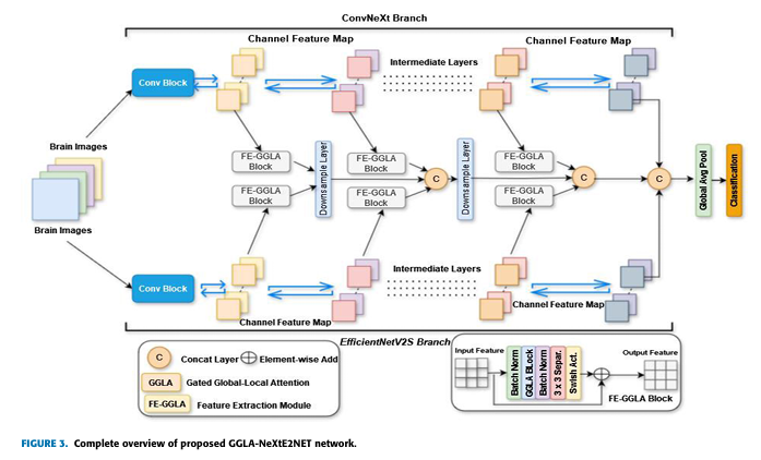
The Dual Branch Ensemble, which the authors abbreviate DBE, runs EfficientNetV2S and ConvNeXt in parallel on the same input. This is not the usual ensembling trick of averaging two predictions. The branches are trained together, and their intermediate feature maps are exchanged through a parameter sharing scheme before either one reaches a classifier.
Why bother with two? Because they see differently. EfficientNetV2S sticks to a fixed 3 by 3 receptive field throughout, which makes it fast and parameter efficient and good at texture. ConvNeXt opens its receptive field as far as 27 by 27, which lets it register that a mass sits at the base of the brain rather than inside the temporal lobe. A meningioma is largely defined by where it is and how it pushes on neighboring tissue. A glioma is largely defined by how its texture bleeds into the tissue around it. Asking one receptive field to do both jobs is asking for a compromise.
Gating instead of choosing
The Gated Global Local Attention module, GGLA, is the piece the paper is named for and the piece worth understanding. Most attention modules in medical imaging pick a lane. Self attention and its relatives model long range dependencies. Convolutional block attention and its relatives model local salience. Combining them usually means concatenating both and hoping the classifier sorts it out.
GGLA instead learns a gate that decides, per feature and per stage, how much of each to let through. The global half is built from two axial passes. Gated Horizontal Attention pools queries along the height axis so that every query point sees its entire row, then Gated Vertical Attention repeats the operation down the columns. Run them in sequence and any pixel can reach any other pixel in two hops, at a fraction of the cost of full self attention over a flattened feature map.
The horizontal pass begins by shrinking the channel dimension and pooling over height.
Mean pooling of the query tensor, with r the channel reduction ratio. The whole point is that the affinity matrix that follows is computed over a single spatial axis rather than over every pixel pair.
Scaled dot product attention then produces the weights, and a softmax normalizes them across the row.
What makes this gated rather than merely axial is the last step. The attended features are folded back into the input through a learnable weight, and then a sigmoid gate decides how much of the result survives.
Equations 23 to 25 of the paper. The sigmoid can suppress an entire attention channel when the global view is unhelpful for a given image, which is exactly what you want when tumor appearance varies this much between patients.
The vertical module mirrors this with its own learnable weight and its own gate. Sequencing them gives the Gated Horizontal Vertical Attention block, GHVA, which is the global half of GGLA.
The local half, and the wrapper around both
Gated Local Attention takes a different route. It stacks a channel wise average pooled map and a max pooled map, pushes them through three 1 by 1 convolutions with Swish activations, and turns the result into a spatial map via softmax. A parallel sigmoid branch computes a gate from the same trunk, and the two are multiplied. The output is a per pixel weighting that says where in this slice the interesting structure sits.
Both halves live inside the FE-GGLA block, which is the unit that actually wraps each backbone stage. Batch normalization, then GGLA, then another batch normalization, then a 3 by 3 separable convolution with Swish, then a 1 by 1 residual connection. Six of these hang off the EfficientNetV2S branch and six off the ConvNeXt branch, and their outputs are concatenated progressively rather than only at the end.
Key takeaway
The design idea worth stealing is not the ensemble, it is the gate. Balancing global and local attention with a learned, per sample gate is cheaper than full self attention and more adaptive than a fixed concatenation. That idea transfers to any imaging task where the useful evidence sometimes lives in the texture and sometimes lives in the anatomy, which describes most of radiology.
The preprocessing stack that does more work than it looks like
Before any of this architecture sees an image, the image has been through six operations. Patch based non local means denoising, wavelet decomposition with coefficient thresholding, a parameterized Wiener filter in the frequency domain, contrast limited adaptive histogram equalization, Laplacian edge enhancement, and a cropping function that removes background skull and air.
Each step has a stated purpose. Non local means handles the speckle that motion introduces during a scan. Wavelet thresholding kills small coefficients that mostly encode noise while preserving the edges that define a tumor boundary. The Wiener step uses the frequency response of the imaging system to pull back structure that denoising smoothed away.
The non local means estimate. Each output pixel is a weighted average of similar patches drawn from across the whole image, not just its immediate neighborhood.
Then comes the augmentation question, and this is where the numbers get interesting. The authors used an Enhanced Super Resolution Generative Adversarial Network to synthesize additional images for the underrepresented classes, 807 for the four class dataset and 1072 for the three class one. Compared against training with no augmentation at all, GAN based augmentation lifted four class accuracy by 2.75% and three class accuracy by 2.64%.
Put that in context. The gap between GGLA-NeXtE2NET at 99.62% and the plain EfficientNetV2S baseline at 97.73% is 1.89 percentage points. The augmentation strategy contributes more than the entire architecture does. That is a real finding and the paper deserves credit for reporting it honestly in Figure 14, but it also means the headline result is as much a statement about data as about network design.
Without augmented data, the model accuracy is lower as can be seen in Figure 14. However, with GAN based augmented data, the model achieves a 2.75% and 2.64% higher accuracy for the 4 class and 3 class brain tumor datasets against non augmented data. Saeed et al., IEEE Access, vol. 13, 2025
What the ablation shows
Ablation studies are usually the least exciting table in a paper and the most trustworthy. This one is well constructed, because it removes one module at a time from the same training setup.
| Variant | Dataset | Accuracy | F1 score | Loss |
|---|---|---|---|---|
| EfficientNetV2S alone | 4 class | 97.73% | 97.72% | 0.078 |
| EfficientNetV2S alone | 3 class | 96.93% | 96.93% | 0.089 |
| DBS-NeXtE2NET, ensemble without GGLA | 4 class | 98.23% | 98.24% | 0.064 |
| DBS-NeXtE2NET, ensemble without GGLA | 3 class | 98.35% | 98.35% | 0.050 |
| GGLA-E2NET, attention without ensemble | 4 class | 98.61% | 98.62% | 0.074 |
| GGLA-E2NET, attention without ensemble | 3 class | 98.11% | 98.10% | 0.048 |
| GGLA-NeXtE2NET, full model | 4 class | 99.62% | 99.62% | 0.014 |
| GGLA-NeXtE2NET, full model | 3 class | 99.06% | 99.06% | 0.015 |
Two things stand out. The first is that the loss drops by a factor of four when both components are present, from 0.064 or 0.074 down to 0.014. That is a much steeper change than the accuracy shift alone would suggest, and it means the full model is not merely getting more answers right, it is far more confident about the ones it gets right.
The second is that the two components are not additive. The ensemble alone buys about half a point. The attention alone buys about nine tenths of a point. Together they buy nearly two. Something about running gated attention across two differently sized receptive fields produces more than the sum, which is a reasonable argument that the architecture is doing real work rather than getting lucky.
Per class performance
| Dataset | Class | Accuracy | Precision | Recall | F1 score |
|---|---|---|---|---|---|
| 4 class | Glioma | 98.98% | 99.49% | 98.99% | 99.24% |
| 4 class | Meningioma | 100% | 99.50% | 100% | 99.75% |
| 4 class | No tumor | 100% | 100% | 100% | 100% |
| 4 class | Pituitary | 99.48% | 99.49% | 99.49% | 99.49% |
| 3 class | Glioma | 98.60% | 99.30% | 98.60% | 98.95% |
| 3 class | Meningioma | 99.28% | 97.89% | 99.29% | 98.58% |
| 3 class | Pituitary | 99.29% | 100% | 99.29% | 99.64% |
The healthy class scores a perfect 100 across every metric on the four class dataset. In one sense that is the easiest class, since a brain with no mass in it looks different from a brain with one. In another sense a perfect score on 200 images should make you want a much larger and more varied set of healthy scans before you believe it, because the healthy class is where a screening tool does most of its work and where a false positive costs a patient an unnecessary contrast study.
The clinical translation gap
Here is where a paper like this meets the thing standing between it and a hospital. Nothing in this section is a criticism of the engineering. It is a description of what a benchmark result can and cannot tell you.
Patient level splitting is the whole ballgame
The three class Figshare dataset contains 3064 T1 weighted contrast enhanced slices, and the paper states plainly that those images come from 233 patients. That works out to roughly thirteen slices per patient. Consecutive slices from the same MRI volume are not independent observations. They show the same tumor from a few millimetres apart, with the same scanner settings, the same patient anatomy, and often the same artifacts.
If the train and test split was made by randomly shuffling images, then slices of the same tumor almost certainly appear on both sides of the split. A model can then score very well by recognizing the patient rather than the pathology. The paper describes an 80, 10, 10 split but does not say whether it was stratified by patient. Until that is confirmed, the 99.06% figure is best read as accuracy on held out slices rather than accuracy on held out patients, and those two quantities can differ by a large margin in medical imaging.
This is not a hypothetical concern invented for this paper. It is the single most common source of inflated results across the whole brain tumor MRI benchmark literature, and it affects nearly every number in the comparison tables, not just this one. Every method listed at 97% or above is subject to the same question.
Synthetic images and where they were allowed to go
The ESRGAN generated images introduce a second version of the same problem. If a synthetic image derived from a real training case ended up in the test split, or if a real image and its synthetic descendant were separated across the split, then the test set is no longer measuring generalization. The paper reports the counts of generated images per class but does not state that synthetic samples were confined to the training partition.
This is straightforward to fix and straightforward to report. One sentence confirming that augmentation happened after the split, and only inside the training fold, would settle it.
Two public datasets are not a population
Both datasets are single source, and both have been circulating in the research community long enough that architectures have quietly been tuned against them. There is no external validation set from a different hospital, a different scanner vendor, or a different acquisition protocol. Field strength, coil configuration, slice thickness, and contrast timing all change how a tumor looks, and a model that has only ever seen one distribution has no way to tell you when it is out of its depth.
Nor are there confidence intervals. With four errors on 793 images, the difference between 99.62% and 99.0% is a handful of images. Reporting a binomial interval, or repeating the experiment across several random seeds, would tell a reader how much of that last percentage point is signal.
Key takeaway
Four errors out of 793 is not the same claim as one error per two hundred patients. The first is a measurement on a specific split of two public datasets. The second is a clinical performance claim that would require patient level splitting, external validation, prospective evaluation, and a defined intended use. The distance between those two statements is where most medical AI research currently sits, and naming it honestly is more useful than another decimal place.
What a hospital would ask for next
Suppose a neuroradiology department wanted to trial this. The questions would arrive in a predictable order. What happens on scans from our scanner, which is not the one in the training data. What is the false negative rate on small lesions specifically, since that is the failure that matters. How does the model behave on a tumor type it was never trained on, a metastasis or a lymphoma, and does it say it does not know or does it confidently pick the closest of three options. What is the calibration, meaning does a 0.95 output actually correspond to being right 95% of the time.
The model as described has no abstention mechanism and no uncertainty estimate. It has four output logits and a softmax. Present it with a class it has never seen and it will return a confident answer from the classes it has. For a screening tool that is a serious design gap, and it is a solvable one. Evidential deep learning and conformal prediction both give a classifier a way to say that an input falls outside what it was trained on, and either would be a natural next step for this architecture. Readers interested in that direction may find our coverage of universal domain adaptation with evidential uncertainty a useful companion, since the same machinery applies whether the unknown class is a radar target or a tumor subtype.
Interpretability, and what Grad-CAM does not prove
The paper includes Grad-CAM heatmaps and derived bounding boxes, and the qualitative comparison against plain EfficientNetV2S is genuinely favourable. The proposed model concentrates its attention on the lesion, while the baseline scatters activation across unrelated tissue.
That is worth something, but it is worth less than it appears. Grad-CAM shows which regions influenced the prediction, not whether the reasoning was clinically sound. A model can attend to the correct lesion and still be keying on an acquisition artifact that happens to co occur with it. Saliency maps have repeatedly been shown to look plausible for models that later fail on shifted data. They are a useful sanity check and a weak form of evidence. The bounding box extraction the authors describe, thresholding the heatmap into a binary mask and fitting boxes to connected components, is a nice engineering addition and points toward the detection work the paper flags as future direction.
How it sits against the field
| Method | Classes | Accuracy | Recall |
|---|---|---|---|
| Modified Vision Transformer, Wang et al. | 4 | 80.78% | 80.00% |
| Pix2Pix conditional GAN with NASNetLarge, Mehmood et al. | 3 | 92.40% | 92.30% |
| Gaussian convolutional neural network, Rizwan et al. | 3 | 97.14% | 97.50% |
| InceptionV3 with DenseNet and EfficientNetV2, Incir and Bozkurt | 4 | 98.41% | 98.50% |
| Ensemble model with LSTM, Islam et al. | 2 | 98.82% | 98.00% |
| Spinal convolution attention network, Tang et al. | 2 | 99.18% | 98.95% |
| Self attention based GAN network, Pandi et al. | 3 | 99.29% | not reported |
| GGLA-NeXtE2NET | 4 | 99.62% | 99.62% |
| GGLA-NeXtE2NET | 3 | 99.06% | 99.05% |
Notice how compressed the top of this table is. Once you exclude the vision transformer result, which the authors themselves point out is an outlier at 80.78%, the field sits between 97% and 99.6%. That is a spread of roughly two and a half points across a decade of architectural work on datasets of a few thousand images. When an entire literature converges into a two point band, the bottleneck has stopped being the model and started being the benchmark.
The training efficiency comparison is the more useful contribution here and gets less attention than it should. The model converges in twenty epochs using Adamax with Swish activations, against thirty to three hundred epochs for the other methods in Table 6. If that holds on larger datasets it matters more for real deployment than the last half point of accuracy, because retraining cost is what determines whether a hospital can update a model when its scanner is replaced. Readers following the compute side of this may want to compare with our piece on why pruning before training can improve generalization, which tackles the same efficiency question from the opposite direction.
Honest limitations
The authors name several themselves, and they are worth restating alongside the ones this analysis has added.
- Resolution dependence. The paper states the model performs optimally when both low and high resolution images are available, and that high quality images may not always be accessible in practice. That is a meaningful constraint given the ESRGAN pipeline sits upstream of everything.
- Centralized training. The current setup requires all data to move to one location, which the authors correctly identify as a privacy problem for multi institution work. They point toward federated approaches as the fix, and that is the right instinct. Our write up on sequential versus parallel federated learning covers the tradeoffs that decision involves.
- Sample size. 7023 images across four classes and 3064 across three classes, from 233 patients in the second case. For a model reporting sub one percent error rates, the test sets are small enough that a few images move the headline figure.
- Dataset bias. Both sources are public, single origin collections. Demographics, scanner vendors, and acquisition protocols are unreported, so there is no way to assess whether performance is even across patient groups.
- No patient level split confirmation. Discussed above, and the most consequential of the open questions.
- No uncertainty output. The model cannot decline to answer, which for a triage or screening role is a design requirement rather than a nice extra.
- Twenty epochs, one run. Fast convergence is a genuine strength, but a single training run with no seed variance reported leaves the stability of the result unmeasured.
None of this makes the work less worth reading. The full text is openly available under a Creative Commons licence, and the paper itself in IEEE Access documents the modules in more detail than most architecture papers manage, including the algorithm listings for GHVA and the full network. It is a solid piece of engineering measured against a benchmark that has largely run out of room.
Conclusion
The core achievement of GGLA-NeXtE2NET is a gating mechanism that lets a network decide, adaptively and per input, how much global context and how much local detail a decision should rest on. That is a cleaner answer to the intra class variation problem than either concatenating both signals or picking one in advance. The ablation supports it, the loss curves support it, and the fact that the ensemble and the attention are more than additive suggests the two are genuinely complementary rather than redundant.
The conceptual shift underneath is small but real. For several years attention design in medical imaging has been a question of which kind of attention to use. Spatial or channel, local or global, convolutional or transformer based. This work reframes it as a question of allocation. Both kinds are available, and the network learns the mixture. That framing survives well beyond brain MRI. Any task where the evidence sometimes lives in fine texture and sometimes in gross anatomy has the same structure, which covers dermoscopy, histopathology, retinal imaging, and chest radiography. The EfficientNetV2L and LightGBM work on skin lesion grading we covered earlier faces exactly this tension in a different modality.
What the paper cannot tell us is how much of the 99.62% survives contact with a new hospital. The datasets are small, single source, and heavily reused. The split protocol is underspecified in the one place where it matters most. There is no external cohort, no uncertainty estimate, and no calibration analysis. These are not unusual omissions, which is precisely the problem. They are standard across the brain tumor MRI literature, and the result is a field where dozens of methods report between 97% and 99.6% on the same few thousand images and nobody can rank them meaningfully.
The productive next steps are visible from here. Confirm the split was made at the patient level and republish the number if it changes. Validate on a cohort from a different scanner. Add an abstention head so the model can flag inputs outside its training distribution. Move to the federated setup the authors already sketch, which solves the privacy constraint and the single source dataset problem at the same time. Extend to detection with the YOLO direction they mention, since a tumor type without a boundary is only half of what a surgeon needs.
Read as an architecture paper, this is good work with a transferable idea at its centre. Read as a clinical claim, it is one careful methodological sentence away from being far more convincing than it currently is. That sentence is worth writing.
Complete PyTorch implementation
The paper implements the model in TensorFlow. Below is a reproducible PyTorch version of the full architecture, written from the module descriptions and the algorithm listings in the paper. It includes the axial gated attention pair, the local attention module, the gated mixture, the FE-GGLA wrapper, the dual branch ensemble, the loss, the Adamax optimizer with the plateau schedule described in the paper, a training loop, an evaluation function that returns a confusion matrix and macro averaged metrics, and a runnable smoke test on dummy tensors.
"""
GGLA-NeXtE2NET
Dual-Branch Ensemble Network with Gated Global-Local Attention
Reference implementation in PyTorch, following Saeed et al., IEEE Access, vol. 13, 2025.

Backbones: EfficientNetV2-S and ConvNeXt-Tiny (torchvision).
Attention: GHA -> GVA (sequential GHVA) for global context, GLA for local spatial context,
           fused by a learned gate inside the GGLA module.
Wrapper:   FE-GGLA block (BN -> GGLA -> BN -> 3x3 separable conv + Swish -> 1x1 residual).
"""

import torch
import torch.nn as nn
import torch.nn.functional as F


# ------------------------------------------------------------------- utilities
class SeparableConv2d(nn.Module):
    """Depthwise 3x3 followed by pointwise 1x1, as used inside the FE-GGLA block."""

    def __init__(self, in_ch, out_ch, kernel_size=3, stride=1, padding=1):
        super().__init__()
        self.depthwise = nn.Conv2d(in_ch, in_ch, kernel_size, stride, padding,
                                   groups=in_ch, bias=False)
        self.pointwise = nn.Conv2d(in_ch, out_ch, kernel_size=1, bias=False)

    def forward(self, x):
        return self.pointwise(self.depthwise(x))


class ChannelLayerNorm(nn.Module):
    """LayerNorm over the channel dimension of an NCHW tensor."""

    def __init__(self, num_channels, eps=1e-6):
        super().__init__()
        self.norm = nn.LayerNorm(num_channels, eps=eps)

    def forward(self, x):
        x = x.permute(0, 2, 3, 1)          # N H W C
        x = self.norm(x)
        return x.permute(0, 3, 1, 2)       # N C H W


# -------------------------------------------------------------- gated attention
class GatedAxialAttention(nn.Module):
    """
    One axis of the gated global attention pair.

    axis="h" gives Gated-Horizontal Attention (GHA). Queries are mean pooled over height so
    every query point sees the whole row. axis="w" gives Gated-Vertical Attention (GVA),
    where pooling happens over width instead. Both end with a sigmoid gate that decides how
    much of the attended signal is allowed back into the residual stream.
    """

    def __init__(self, channels, reduction=8, axis="h"):
        super().__init__()
        assert axis in ("h", "w")
        self.axis = axis
        self.inner = max(channels // reduction, 8)

        self.norm = ChannelLayerNorm(channels)
        self.to_q = nn.Conv2d(channels, self.inner, 1, bias=False)
        self.to_k = nn.Conv2d(channels, self.inner, 1, bias=False)
        self.to_v = nn.Conv2d(channels, self.inner, 1, bias=False)
        self.project = nn.Conv2d(self.inner, channels, 1, bias=False)

        # gate branch, equations 24 and 25 of the paper
        self.gate = nn.Conv2d(channels, channels, 1, bias=True)
        # learnable residual weight, alpha for GHA and beta for GVA
        self.weight = nn.Parameter(torch.zeros(1))
        self.scale = self.inner ** -0.5

    def forward(self, x):
        n, c, h, w = x.shape
        xn = self.norm(x)
        q, k, v = self.to_q(xn), self.to_k(xn), self.to_v(xn)

        if self.axis == "h":
            # pool over height, attention runs along the width axis of every row
            q = q.mean(dim=2)                       # N Ci W
            k = k.mean(dim=2)                       # N Ci W
            v = v.mean(dim=2)                       # N Ci W
            affinity = torch.einsum("ncx,ncy->nxy", q, k) * self.scale
            attn = affinity.softmax(dim=-1)         # N W W
            out = torch.einsum("nxy,ncy->ncx", attn, v)     # N Ci W
            out = out.unsqueeze(2).expand(n, self.inner, h, w)
        else:
            q = q.mean(dim=3)                       # N Ci H
            k = k.mean(dim=3)
            v = v.mean(dim=3)
            affinity = torch.einsum("ncx,ncy->nxy", q, k) * self.scale
            attn = affinity.softmax(dim=-1)         # N H H
            out = torch.einsum("nxy,ncy->ncx", attn, v)     # N Ci H
            out = out.unsqueeze(3).expand(n, self.inner, h, w)

        out = self.project(out.contiguous())
        y = self.weight * out + x                   # equations 23 and 28
        return torch.sigmoid(self.gate(y)) * y      # gated output


class GatedHorizontalVerticalAttention(nn.Module):
    """GHVA. Horizontal pass, then vertical pass, so each pixel reaches every other pixel."""

    def __init__(self, channels, reduction=8):
        super().__init__()
        self.gha = GatedAxialAttention(channels, reduction, axis="h")
        self.gva = GatedAxialAttention(channels, reduction, axis="w")

    def forward(self, x):
        return self.gva(self.gha(x))


class GatedLocalAttention(nn.Module):
    """
    GLA. Average and max pooled channel descriptors are stacked, passed through three
    1x1 convolutions with Swish, turned into a spatial map by softmax, and multiplied by a
    sigmoid gate computed from the same trunk.
    """

    def __init__(self, hidden=16):
        super().__init__()
        self.trunk = nn.Sequential(
            nn.Conv2d(2, hidden, 1, bias=False), nn.SiLU(),
            nn.Conv2d(hidden, hidden, 1, bias=False), nn.SiLU(),
            nn.Conv2d(hidden, 1, 1, bias=False),
        )
        self.gate = nn.Conv2d(1, 1, 1, bias=True)

    def forward(self, x):
        n, c, h, w = x.shape
        avg_map = x.mean(dim=1, keepdim=True)
        max_map = x.amax(dim=1, keepdim=True)
        stacked = torch.cat([avg_map, max_map], dim=1)
        trunk = self.trunk(stacked)                          # N 1 H W
        weights = trunk.flatten(2).softmax(dim=-1).view(n, 1, h, w) * (h * w)
        gate = torch.sigmoid(self.gate(trunk))
        return x * (weights * gate)


class GGLA(nn.Module):
    """
    Gated Global-Local Attention. The global path is GHVA, the local path is GLA, and a
    learned per channel gate decides the mixture instead of fixing it by hand.
    """

    def __init__(self, channels, reduction=8):
        super().__init__()
        self.global_path = GatedHorizontalVerticalAttention(channels, reduction)
        self.local_path = GatedLocalAttention()
        self.mix_gate = nn.Sequential(
            nn.AdaptiveAvgPool2d(1),
            nn.Conv2d(channels * 2, max(channels // 4, 8), 1), nn.SiLU(),
            nn.Conv2d(max(channels // 4, 8), channels, 1), nn.Sigmoid(),
        )

    def forward(self, x):
        g = self.global_path(x)
        l = self.local_path(x)
        gate = self.mix_gate(torch.cat([g, l], dim=1))
        return gate * g + (1.0 - gate) * l


class FEGGLA(nn.Module):
    """Feature-Enhanced GGLA block, the unit that wraps every backbone stage output."""

    def __init__(self, in_ch, out_ch, reduction=8):
        super().__init__()
        self.bn_in = nn.BatchNorm2d(in_ch)
        self.ggla = GGLA(in_ch, reduction)
        self.bn_mid = nn.BatchNorm2d(in_ch)
        self.sep = SeparableConv2d(in_ch, out_ch)
        self.act = nn.SiLU()
        self.skip = nn.Conv2d(in_ch, out_ch, 1, bias=False)

    def forward(self, x):
        y = self.ggla(self.bn_in(x))
        y = self.act(self.sep(self.bn_mid(y)))
        return y + self.skip(x)


# --------------------------------------------------------------- full ensemble
class GGLANeXtE2NET(nn.Module):
    """
    Dual-Branch Ensemble Network. EfficientNetV2-S keeps a fixed 3x3 receptive field, while
    ConvNeXt widens up to 27x27, so the two branches disagree in a useful way before the
    concatenated features reach the classifier.
    """

    def __init__(self, num_classes=4, embed=256, pretrained=False, dropout=0.3):
        super().__init__()
        from torchvision.models import (efficientnet_v2_s, convnext_tiny,
                                        EfficientNet_V2_S_Weights, ConvNeXt_Tiny_Weights)

        eff_w = EfficientNet_V2_S_Weights.DEFAULT if pretrained else None
        cnx_w = ConvNeXt_Tiny_Weights.DEFAULT if pretrained else None
        self.eff_stages = nn.ModuleList(efficientnet_v2_s(weights=eff_w).features)
        self.cnx_stages = nn.ModuleList(convnext_tiny(weights=cnx_w).features)

        # stage indices whose outputs are refined by an FE-GGLA block
        self.eff_taps = [2, 4, 6]
        self.cnx_taps = [1, 3, 5]
        eff_dims, cnx_dims = self._probe_dims()

        self.eff_blocks = nn.ModuleList([FEGGLA(d, embed) for d in eff_dims])
        self.cnx_blocks = nn.ModuleList([FEGGLA(d, embed) for d in cnx_dims])

        fused = embed * (len(eff_dims) + len(cnx_dims))
        self.fuse = nn.Sequential(
            nn.Conv2d(fused, embed * 2, 1, bias=False),
            nn.BatchNorm2d(embed * 2), nn.SiLU(),
        )
        self.pool = nn.AdaptiveAvgPool2d(1)
        self.head = nn.Sequential(nn.Flatten(), nn.Dropout(dropout),
                                  nn.Linear(embed * 2, num_classes))

    @torch.no_grad()
    def _probe_dims(self):
        dummy = torch.zeros(1, 3, 128, 128)
        eff_dims, x = [], dummy
        for i, stage in enumerate(self.eff_stages):
            x = stage(x)
            if i in self.eff_taps:
                eff_dims.append(x.shape[1])
        cnx_dims, x = [], dummy
        for i, stage in enumerate(self.cnx_stages):
            x = stage(x)
            if i in self.cnx_taps:
                cnx_dims.append(x.shape[1])
        return eff_dims, cnx_dims

    def _run_branch(self, x, stages, taps, blocks):
        feats, bi = [], 0
        for i, stage in enumerate(stages):
            x = stage(x)
            if i in taps:
                feats.append(blocks[bi](x))
                bi += 1
        return feats

    def forward(self, x):
        eff_feats = self._run_branch(x, self.eff_stages, self.eff_taps, self.eff_blocks)
        cnx_feats = self._run_branch(x, self.cnx_stages, self.cnx_taps, self.cnx_blocks)
        target = eff_feats[-1].shape[-2:]
        pooled = [F.adaptive_avg_pool2d(f, target) for f in eff_feats + cnx_feats]
        fused = self.fuse(torch.cat(pooled, dim=1))
        return self.head(self.pool(fused))


# ---------------------------------------------------------------------- losses
class LabelSmoothedCrossEntropy(nn.Module):
    """Categorical cross entropy, the loss the paper reports, with optional smoothing."""

    def __init__(self, smoothing=0.0):
        super().__init__()
        self.smoothing = smoothing

    def forward(self, logits, targets):
        return F.cross_entropy(logits, targets, label_smoothing=self.smoothing)


# ------------------------------------------------------- train and evaluate
def train_one_epoch(model, loader, optimizer, criterion, device):
    model.train()
    running, seen, correct = 0.0, 0, 0
    for images, labels in loader:
        images, labels = images.to(device), labels.to(device)
        optimizer.zero_grad(set_to_none=True)
        logits = model(images)
        loss = criterion(logits, labels)
        loss.backward()
        optimizer.step()
        running += loss.item() * labels.size(0)
        correct += (logits.argmax(1) == labels).sum().item()
        seen += labels.size(0)
    return running / seen, correct / seen


@torch.no_grad()
def evaluate(model, loader, criterion, device, num_classes):
    model.eval()
    running, seen = 0.0, 0
    confusion = torch.zeros(num_classes, num_classes, dtype=torch.long)
    for images, labels in loader:
        images, labels = images.to(device), labels.to(device)
        logits = model(images)
        running += criterion(logits, labels).item() * labels.size(0)
        preds = logits.argmax(1)
        for t, p in zip(labels.view(-1), preds.view(-1)):
            confusion[t.long(), p.long()] += 1
        seen += labels.size(0)

    tp = confusion.diag().float()
    support = confusion.sum(1).float()
    predicted = confusion.sum(0).float()
    precision = torch.where(predicted > 0, tp / predicted.clamp(min=1), torch.zeros_like(tp))
    recall = torch.where(support > 0, tp / support.clamp(min=1), torch.zeros_like(tp))
    denom = (precision + recall).clamp(min=1e-8)
    f1 = 2 * precision * recall / denom
    return {
        "loss": running / seen,
        "accuracy": (tp.sum() / support.sum()).item(),
        "macro_precision": precision.mean().item(),
        "macro_recall": recall.mean().item(),
        "macro_f1": f1.mean().item(),
        "confusion": confusion,
    }


def build_optimizer(model, lr=1e-3):
    """Adamax with the ReduceLROnPlateau schedule the paper describes."""
    optimizer = torch.optim.Adamax(model.parameters(), lr=lr)
    scheduler = torch.optim.lr_scheduler.ReduceLROnPlateau(
        optimizer, mode="min", factor=0.5, patience=1)
    return optimizer, scheduler


# ------------------------------------------------------------------ smoke test
if __name__ == "__main__":
    from torch.utils.data import TensorDataset, DataLoader

    torch.manual_seed(0)
    device = torch.device("cuda" if torch.cuda.is_available() else "cpu")
    num_classes = 4

    model = GGLANeXtE2NET(num_classes=num_classes, embed=64, pretrained=False).to(device)
    params = sum(p.numel() for p in model.parameters()) / 1e6
    print(f"parameters {params:.1f} M")

    images = torch.randn(16, 3, 128, 128)
    labels = torch.randint(0, num_classes, (16,))
    loader = DataLoader(TensorDataset(images, labels), batch_size=8, shuffle=True)

    criterion = LabelSmoothedCrossEntropy(smoothing=0.05)
    optimizer, scheduler = build_optimizer(model, lr=1e-3)

    for epoch in range(2):
        loss, acc = train_one_epoch(model, loader, optimizer, criterion, device)
        stats = evaluate(model, loader, criterion, device, num_classes)
        scheduler.step(stats["loss"])
        print(f"epoch {epoch}  train loss {loss:.4f}  train acc {acc:.3f}  "
              f"val acc {stats['accuracy']:.3f}  macro f1 {stats['macro_f1']:.3f}")

    print("confusion matrix")
    print(stats["confusion"])
    print("smoke test finished")
Running the file as a script builds the model, reports its parameter count, trains for two epochs on random tensors, and prints a confusion matrix. It is a structural check rather than a reproduction of the published numbers, which would need the actual datasets, the full preprocessing pipeline, and pretrained backbone weights.
Frequently asked questions
What does GGLA-NeXtE2NET actually do differently from other brain tumor classifiers?
It runs two convolutional backbones in parallel, EfficientNetV2S with a fixed small receptive field and ConvNeXt with a much wider one, and refines the features from both using a gated attention block. The gate learns how much global context and how much local detail each decision should use, rather than fixing that balance in the architecture. That adaptivity is the main novelty.
Is 99.62% accuracy good enough for clinical use?
No, and accuracy alone is the wrong question. The figure comes from one split of two public datasets with no external validation, no patient level split confirmation, no confidence intervals, and no uncertainty output. Clinical deployment requires prospective evaluation on data from the target hospital, a defined intended use, regulatory clearance, and a mechanism for the model to flag cases it cannot handle. None of that is present yet.
Why does patient level data splitting matter so much?
The three class Figshare dataset holds 3064 MRI slices taken from only 233 patients, which is roughly thirteen slices per patient. Slices from the same scan are highly correlated. If the split was made by shuffling images rather than patients, near duplicate views of the same tumor land in both training and test data, and the model can score well by recognizing the patient instead of the pathology. The paper does not state which method was used.
How much of the performance comes from the architecture and how much from data preparation?
Roughly comparable amounts. The full model beats the plain EfficientNetV2S baseline by 1.89 percentage points on the four class dataset. Switching from no augmentation to ESRGAN based synthetic augmentation is worth 2.75 percentage points on the same dataset. The six stage denoising pipeline contributes on top of that. Data preparation is doing at least as much work as the network design.
Can this model detect where the tumor is, not just what type it is?
Only indirectly. The authors apply Grad-CAM to produce heatmaps, threshold those into binary masks, and fit bounding boxes to the connected components. That gives an approximate localization derived from a classifier, not a trained detector. The paper names object detection with a YOLO style model as future work, which would give proper boundaries suitable for surgical planning.
Where can I get the datasets used in the paper?
Both are public. The four class set is the Brain Tumor MRI Dataset published by Masoud Nickparvar on Kaggle, with 7023 images across glioma, meningioma, pituitary tumor, and no tumor. The three class set is the Brain Tumor Dataset published by Jun Cheng on Figshare, with 3064 contrast enhanced T1 weighted slices from 233 patients.
Read the full paper and pull the datasets to reproduce the results yourself.
A. Saeed, K. Shehzad, S. S. Bhatti, S. Ahmed, and A. T. Azar, “GGLA-NeXtE2NET: A Dual-Branch Ensemble Network With Gated Global-Local Attention for Enhanced Brain Tumor Recognition,” IEEE Access, vol. 13, pp. 7234 to 7257, 2025, doi 10.1109/ACCESS.2025.3525518. Published under a Creative Commons Attribution 4.0 licence.
This analysis is based on the published paper and an independent evaluation of its claims.
Pingback: FixMatch: Simplified SSL Breakthrough - aitrendblend.com