
- Diabetic retinopathy
- Mobile health
- Teleophthalmology
- Transfer learning
- Fundus imaging
- Clinical validation
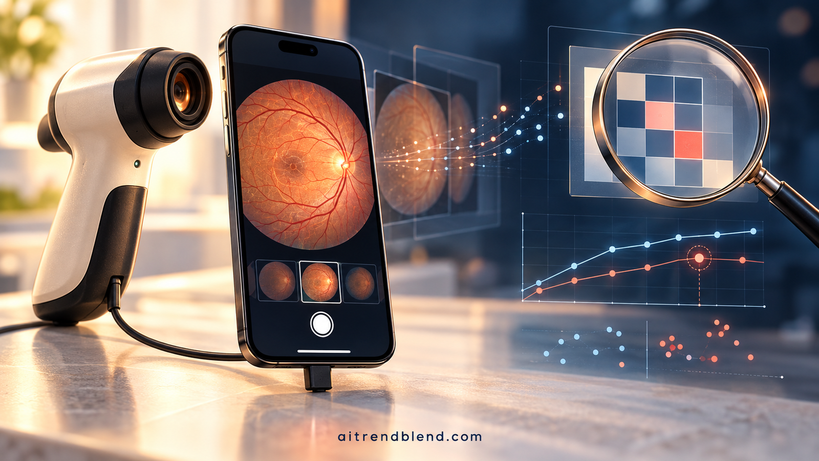
A nurse on a medical caravan outside Fez presses a handheld retinal camera against a patient’s eye, taps a phone screen and waits. About a second later the app answers that diabetic retinopathy is present, with 90 percent confidence. The patient has diabetes, lives far from the nearest ophthalmologist, and is one of about 1.5 million people with diabetes in the region, a number the authors expect to reach 2.6 million by 2030.
That scene is the premise of a 2025 paper in Intelligence-Based Medicine from El-Mehdi Chakour and colleagues at Sidi Mohamed Ben Abdellah University in Fez and ESIEE Paris. It reports accuracies between 90.90 and 98.61 percent. A screening tool that errs in the wrong direction can cost someone their sight, so this article does what the abstract does not invite. It rebuilds the headline metrics from the paper’s own confusion matrices, and several of the published numbers do not survive the exercise.
Key points
- The paper combines a handheld nonmydriatic camera, a Gaussian, CLAHE and gamma enhancement chain and a fine tuned DenseNet-121 inside an Android app to flag diabetic retinopathy as present or absent.
- Recomputed from the paper’s Table 6, EyePACS specificity is 87.9 percent, not the 99.40 percent printed in Table 4. In plain terms, 121 of 1000 healthy test images were flagged as disease.
- The APTOS confusion matrix labelled DenseNet-121 matches the Inception v3 column of Table 4, and it holds 918 images although the stated test set has 959.
- Every F1 score in Table 4 sits near 70, which cannot be true when precision and sensitivity sit near 98. The correct F1 values are around 98 for the private set.
- Each test set is ten percent of an augmented image pool, and no model is ever tested on a dataset it was not trained on.
- The abstract’s 162.5 ms is not a phone measurement. The phone measurement in the text is 1.2 seconds per image.
This article is an educational analysis of a published research paper. It is not medical advice. The system it discusses is a research prototype and not an approved medical device, and nothing here should be used to diagnose, screen for or treat any condition. Anyone concerned about diabetic eye disease should speak with a qualified eye care professional.
Why screening has to leave the clinic
Diabetic retinopathy damages the small blood vessels of the retina. The earliest visible signs are microaneurysms, tiny bulges in weakened capillaries. They can rupture into hemorrhages, and leaking vessels leave soft and hard exudates, the lipid deposits that mark more advanced disease. Treatment works best when the disease is caught early, which is why screening programs photograph the back of the eye long before a patient notices any loss of vision.
The burden is large. The paper quotes prevalence figures of 35.9 percent in Africa, 32.9 percent in the Middle East and North Africa and 33.3 percent in North America among people with diabetes, drawing on a global systematic review by Teo and colleagues in Ophthalmology. Its introduction also says that 700 million people could have diabetes by 2025. The review it cites projects burden through 2045, so that date looks like a slip and is worth checking before anyone repeats it.
The access problem in the authors’ own region is stark. They report only 330 ophthalmologists in the Moroccan public sector, with more than 80 percent of private sector ophthalmologists concentrated on the Casablanca Kenitra axis. Handheld retinal cameras that clip onto a phone look like a natural answer, and earlier studies cited in the paper compared several of them against tabletop cameras, including work by Midena and colleagues in the Journal of Clinical Medicine and by Lu and colleagues in PLOS Digital Health. One cited study of an AI system on a handheld camera, from Rogers and colleagues, reported AUROC values of 89.4 and 94.3 percent for referable and proliferative disease. Our wider coverage of medical imaging and diagnostic AI follows the same arc from tabletop systems to the field.
What the system actually does
The pipeline has four parts. Images come from an oDocs Nun IR camera, a portable nonmydriatic device with a resolution of 2880 by 2160 pixels and a field of view of 45 to 55 degrees, which attaches to an Android phone. Each image is resized, split into red, green and blue channels, and enhanced by one of five candidate filter chains. The winning chain applies a Gaussian filter, then CLAHE, a local contrast method, then adaptive gamma correction, which brightens or darkens an image through a power law.
The enhanced image is resized to 224 by 224 pixels and passed to a DenseNet-121 pretrained on natural images and fine tuned for a binary question, diabetic retinopathy or none. The authors train for up to 200 epochs with RMSProp at a learning rate of 0.001, binary cross entropy, a dropout layer and a sigmoid output, and stop early after 50 epochs without a gain in validation accuracy. The trained model is converted to TensorFlow Lite and wrapped in an Android app that talks to a server, so that tablets and desktops at a hospital can see the results.
One note on vocabulary. The paper calls its chains of filters blockchains, and the header of its Table 2 does too. The word has nothing to do with a distributed ledger here. It simply means a sequence of processing steps. For deployment constraints such as model size and speed, our model compression coverage covers the techniques a team like this would reach for next.
The data behind the numbers
Three datasets feed the study. APTOS and EyePACS are public Kaggle collections. The private dataset was collected at CHU Hassan II in Fez with the oDocs camera during mobile screening campaigns in rural and semi urban areas. Three ophthalmologists labelled it independently on a five stage scale, with a fourth expert resolving disagreements, which is a sound labelling protocol. The five stages were then collapsed into two classes, no retinopathy and retinopathy.
| Dataset | Original images | Images kept | After augmentation | Train, validation, test |
|---|---|---|---|---|
| Private | 1321 | 1321 | 7200 | 5400, 1080, 720 |
| APTOS | 3662 | 2880 | 9566 | 7174, 1433, 959 |
| EyePACS | 35126 | 4290 | 20000 | 15000, 3000, 2000 |
The table already raises questions. The private set is small, with only 94 images at the proliferative stage, and about 80.6 percent of its labelled images show retinopathy once the four diseased stages are merged. The paper’s counts also disagree slightly with themselves, since the stage counts add up to 1319 images while Table 3 of the paper says 1321. For the public sets the authors dropped images with artifacts, keeping 78.6 percent of APTOS and only 12.2 percent of EyePACS. For a system meant to cope with blurry, badly lit handheld images, discarding the hardest public images is a curious choice, and the paper does not report how the model behaves on poor quality input.
Rebuilding the results from the confusion matrices
Table 6 of the paper gives the confusion matrix for each dataset, which is the raw count of correct and incorrect calls for each class. Every standard screening metric can be recomputed from it with four formulas.
Sensitivity is the share of diseased eyes that the system catches. Specificity is the share of healthy eyes it correctly clears. For a screening tool, sensitivity decides who is missed and specificity decides how many healthy people are sent for an unnecessary referral. The table below sets the values printed in Table 4 of the paper beside the values recomputed from Table 6.
| Dataset | Metric | Printed in the paper | Recomputed from matrix |
|---|---|---|---|
| Private | Accuracy | 98.61 | 98.61 |
| Sensitivity | 98.33 | 98.33 | |
| Specificity | 100.00 | 98.89 | |
| Precision | 98.88 | 98.88 | |
| F1 score | 70.03 | 98.61 | |
| APTOS | Accuracy | 98.03 | 97.39 |
| Sensitivity | 97.76 | 97.10 | |
| Specificity | 99.78 | 97.66 | |
| Precision | 98.20 | 97.53 | |
| F1 score | 67.98 | 97.32 | |
| EyePACS | Accuracy | 90.90 | 90.90 |
| Sensitivity | 93.90 | 93.90 | |
| Specificity | 99.40 | 87.90 | |
| Precision | 88.58 | 88.58 | |
| F1 score | 69.37 | 91.17 |
Accuracy, sensitivity and precision on the private and EyePACS sets reproduce exactly, which is reassuring about the confusion matrices themselves. The trouble sits in the other entries.
A specificity that cannot be right
On the private set, the matrix shows 356 healthy images cleared and 4 flagged, which gives a specificity of 98.89 percent, while Table 4 prints 100.00. The EyePACS gap is far larger. The matrix shows 879 healthy images cleared and 121 flagged, a specificity of 87.9 percent, against a printed 99.40. The two cannot both hold. Sensitivity on that set, 939 of 1000, is genuinely good, but the system also sends about one in eight healthy eyes for follow up, and a reader who trusts Table 4 would never learn that.
The APTOS matrix that seems to belong to another model
The APTOS matrix is odder still. It lists 459 and 11 for healthy eyes and 13 and 435 for diseased eyes. Those four numbers add up to 918, not the 959 test images the paper states, so 41 images are unaccounted for. They also give an accuracy of 97.39 percent, which matches the 97.38 percent in the abstract and the results text, but not the 98.03 percent in Table 4 and the conclusion. The table below shows where those figures come from.
| Metric | DenseNet-121, Table 4 | Inception v3, Table 4 | Recomputed from matrix |
|---|---|---|---|
| Accuracy | 98.03 | 97.38 | 97.39 |
| Sensitivity | 97.76 | 97.09 | 97.10 |
| Precision | 98.20 | 97.53 | 97.53 |
| Specificity | 99.78 | 100.00 | 97.66 |
Three of the four recomputed values line up with the Inception v3 column to within rounding, and none line up with the DenseNet-121 column. Specificity matches neither. The simplest reading is that the APTOS matrix came from a different model or run than the one the paper calls its best. I cannot tell from the paper which it was, and the authors are the ones who can settle it. The practical effect is that the abstract’s 97.38 percent and the conclusion’s 98.03 percent describe the same system on the same dataset and cannot both be correct.
An F1 score that cannot exist
Every F1 score in Table 4 sits between roughly 66 and 70, including 70.03 for DenseNet-121 on the private set. F1 is the harmonic mean of precision and sensitivity, so it must fall between those two numbers or very near them. With a precision of 98.88 percent and a sensitivity of 98.33 percent on the same row, the F1 has to be about 98.6 percent. The recomputed values in Table 2 confirm it. These figures look like a different quantity under the F1 label, perhaps a score averaged in a way the paper does not explain.
When a paper prints both a confusion matrix and a metrics table, recompute one from the other. In this paper accuracy, sensitivity and precision survive that check on two datasets, while specificity, the APTOS column and every F1 score do not. A recomputation like this takes minutes and is the cheapest form of review a reader can do.
Balanced test sets and what a clinic would actually see
The EyePACS test set contains exactly 1000 healthy and 1000 diseased images, and the private test set holds 360 of each. Real screening populations are not balanced. Among the full EyePACS collection described in the paper, 9316 of 35126 images, about 26.5 percent, show some retinopathy. A screening tool’s usefulness to a patient depends on the positive predictive value, the chance that a flagged patient truly has the disease, and that value falls as prevalence falls.
Take the EyePACS sensitivity of 93.9 percent and the recomputed specificity of 87.9 percent, and suppose a clinic sees the same 26.5 percent prevalence as the full collection. This is my own illustrative arithmetic, not a result in the paper. The positive predictive value comes out near 73.7 percent, so about one flagged patient in four would be a false alarm, against about 11 percent in the balanced test set the paper reports. The negative predictive value in the same setting is about 97.6 percent. If Table 4’s 99.40 percent specificity were true, the false alarm rate would be far lower. This is why specificity matters, and why its misreporting matters in a screening paper.
Augmentation, splits and the test set
The paper states plainly that augmentation was applied only to the training set after the data were partitioned, so no augmented image can appear in validation or test data. The numbers in Table 1 are hard to square with that statement. For every dataset the test set is exactly ten percent of the post augmentation total, 720 of 7200, 959 of 9566 and 2000 of 20000. If the split came first, the test sets would be ten percent of the original images and could not contain 2000 images drawn from only 4290 EyePACS originals with a balanced 1000 and 1000 mix.
The likelier explanation is that images were augmented first, then split, so rotated or flipped copies of the same retina can sit on both sides of the split. The paper does not say, and it does not mention splitting by patient either. EyePACS contains both eyes of each patient, and the private set may hold several images per patient. Leakage of this kind inflates accuracy and cannot be detected from the paper. Table 5 of the paper reports a validation accuracy of 93.92 percent on EyePACS, yet the test accuracy is 90.90 percent, a three point gap on supposedly matched data that deserves an explanation.
Does the preprocessing help
The enhancement study compares five filter chains using three image quality measures. SSIM and PSNR compare the enhanced image with the original, and RCEF measures how much contrast increased.
| Chain | Filters | SSIM | PSNR | RCEF |
|---|---|---|---|---|
| 1 | MF + CLAHE + AGC | 0.9804 | 33.2531 | 1.0177 |
| 2 | GF + CLAHE + AGC | 0.9808 | 33.2950 | 1.0476 |
| 3 | BF + CLAHE + AGC | 0.9803 | 33.2317 | 1.0378 |
| 4 | NLM + CLAHE + AGC | 0.9804 | 33.2096 | 1.0381 |
| 5 | MMF + CLAHE + AGC | 0.9802 | 33.2641 | 1.0276 |
Three problems stand out. First, the differences are tiny. SSIM spans 0.0006 across the five chains and PSNR spans less than 0.09 decibels, and no repeated measurement or confidence interval is given. Second, higher SSIM and PSNR mean the enhanced image stays closer to the original. Selecting for those measures favors the chain that changes the image least, which is an odd target for a method whose purpose is to improve visibility. Third, the paper says the preprocessing contributes to improved model accuracy across all datasets, yet it never trains a model on unprocessed images for comparison. The benefit of the chain for classification is asserted and not measured. The text also says the MMF filter performed poorly and its results are not shown, while chain 5 in the table is built on it.
Real time on a phone
The abstract promises an average processing time of 162.5 ms on mobile devices, and the conclusion repeats a figure of 161.62 ms per image. That number is the DenseNet-121 entry for the private dataset in Table 7, a benchmark of model depth, memory and inference time that sits beside other models. The same DenseNet-121 appears there with 210.03 ms on APTOS and 137.52 ms on EyePACS, although input size and architecture are identical, and 162.5 does not match any entry or their mean of about 169.7. The paper does not say what hardware produced the table.
The measurement on actual smartphones appears later, in Section 4.6, where the authors report an average of 1.2 seconds per image including preprocessing and prediction, timed across 100 test images. That is about 7.4 times the abstract’s figure. A second per image is still comfortable for a nurse in a consultation, so the clinical claim survives. The headline number does not describe the phone, and the paper never reports whether the converted TensorFlow Lite model reproduces the accuracy of the Keras model on the workstation. Table 7 also lists MobileNetV2 with a larger memory size than DenseNet-121 under unstated units, while the text argues that DenseNet has fewer parameters, so that table is worth a second look before anyone cites it.
Generalization across datasets
The abstract says the model is trained using a private dataset along with two large public datasets, and the text repeatedly praises generalization across heterogeneous data. The training curves in the paper show a separate run for each dataset, with different numbers of epochs, and every result is a test on a split of the same dataset used for training. Nowhere does the paper train on one source and test on another. That is the experiment that would show whether a model built on tabletop camera images survives handheld ones, and the paper does not contain it.
…has only been tested by us and a few members of the medical staff. Chakour and colleagues, Intelligence-Based Medicine 12, 2025, on the app’s current status
The authors are frank about this elsewhere. They state that the app has so far been tested only by the research team and a few medical staff, that validation by the authorities and a field campaign in the Fez region are still to come, and that these devices must only be used under the full responsibility of healthcare professionals. They also list uncertainty estimation as future work, a topic we cover in our analysis of subclass learning for uncertainty estimation. Those admissions are the right frame for reading the accuracy tables.
Smaller slips worth knowing
None of these changes the picture alone, though together they argue for careful reading and for checking before citing.
- The Figure 8 legend for the private dataset assigns an AUROC of 0.9991 to Inception v3 and 0.9945 to DenseNet-121, the reverse of Table 7.
- The paper expands the acronym AMD as Assisted Mobile Diagnostic and also uses MAD for Mobile Aided Diagnosis, while AMD also stands for age related macular degeneration in the same text.
- The app is described as written in JavaScript in one paragraph and in Java inside Android Studio in another.
- The EyePACS sampling section lists 1534 and 2764 images, which add to 4298, while Table 3 says 4290.
- Reference 20 is a remote sensing change detection paper but is cited for transfer learning on diabetic retinopathy images, and the related work text attributes a CLAHE study to reference 18 while the list gives that number to a different article.
- References 11 and 12 are about autism, cited in a sentence on retinopathy detection, and reference 48, cited for split ratios, is marked as retracted in the reference list.
- The comparison in Table 8 sets results on different datasets, splits and tasks side by side, including multi class and binary problems, so the ranking it implies is not a controlled comparison.
The clinical translation gap
A research prototype and a screening service sit a long way apart, and this paper covers only the first steps. Several gaps would need to close before a program could use anything like it.
The first is validation on the right population. A model must be tested on images from other cameras, clinics and patients, split by patient so that no eye appears on both sides, with confidence intervals around every metric. The second is staging. The paper’s aim is early detection, particularly mild disease, yet it reports only the binary result. A sensitivity figure broken down by stage would show how well the earliest disease is caught, which is where screening earns its value.
The third is image quality. Handheld images are often blurred or badly lit, the authors say so, and a deployed system needs a way to flag an ungradable image instead of returning a confident answer. The prototype shows a single confidence figure and no such check. The fourth is the operating point. A screening program must choose a threshold that balances missed disease against unnecessary referrals, and report the resulting positive and negative predictive values at the prevalence of its own population. The fifth is regulation and workflow. Approval by the relevant authorities, clear rules for who acts on a positive result, how referrals travel to a hospital such as the pilot site in Fez, and how patient data are protected all stand outside the model. The paper describes encryption, anonymization and informed consent for its private dataset, which is good practice, and it correctly says that clinicians must remain responsible for decisions.
Clinical limitations
The study has limits that readers should weigh against its headline numbers. The private dataset has 1319 labelled images from one hospital, one camera model and a population of adults with confirmed diabetes, and it excludes patients with other retinal disease, which real screening populations include. Its largest stage group is minimal disease with 381 images and its smallest is proliferative disease with 94, so stage level conclusions would rest on very few cases.
The public datasets were filtered for quality, which removes most of the difficult images, and only one split is reported even though the method section mentions five fold cross validation. There are no repeated runs, no intervals and no tests of statistical significance for the differences between architectures. The private data are not available, so outside groups cannot repeat the key experiments. The three datasets were also relabelled into two classes, which hides performance on the mild stage, and none of the results is a prospective clinical trial. These are ordinary limits for a first prototype. They are also the reasons the reported numbers should be read as promising and unproven.
What this means for readers and builders
For people reading medical AI papers, the lesson is procedural. Recompute whatever can be recomputed. Check that the test set is independent of the training set and that the reported counts add up. Ask what the prevalence in the test data was, and what it will be in practice. A paper can have a sensible clinical idea and a useful dataset while its tables still carry errors, and both things can be said at once.
For teams building similar tools, the paper offers a usable starting point. A DenseNet-121 backbone, a modest enhancement chain, a phone app and a hospital pilot site are all reasonable. The next steps are the unglamorous ones, a patient level split, an external test on handheld images, stage level sensitivity, an ungradable image detector and a prevalence adjusted evaluation.
The idea of low cost point of care screening for diabetic retinopathy is sound and the authors’ dataset work looks valuable. The reported performance is not yet trustworthy as printed, because the paper’s own tables disagree on specificity, on the APTOS results and on the F1 scores.
Complete PyTorch implementation
The code below is a reference implementation written for this article, an independent reading of the pipeline in PyTorch although the authors used Keras. It includes the enhancement chain, a DenseNet-121 classifier, the training loop, and a metrics function that works directly from a confusion matrix, so you can repeat the audit above. The smoke test recomputes the paper’s Table 6 and then runs the model on dummy images. It is research code and not a medical device.
"""
Mobile DR screening pipeline, an independent reading of Chakour et al.,
Intelligence-Based Medicine 12 (2025) 100259. Written for aitrendblend.com.
Research and teaching code only. It is not a medical device and has not been clinically validated.
"""
import numpy as np
import cv2
import torch
import torch.nn as nn


# ----------------------------------------------------------------------------
# 1. Enhancement chain 2 from the paper, Gaussian filter then CLAHE then adaptive gamma
# ----------------------------------------------------------------------------
def enhance_fundus(bgr, sigma=1.5, clip_limit=2.0, tile=8):
    """bgr is a uint8 image of shape H x W x 3. The paper gives no parameter values, these are defaults."""
    blurred = cv2.GaussianBlur(bgr, (0, 0), sigma)
    lab = cv2.cvtColor(blurred, cv2.COLOR_BGR2LAB)
    clahe = cv2.createCLAHE(clipLimit=clip_limit, tileGridSize=(tile, tile))
    lab[..., 0] = clahe.apply(lab[..., 0])
    eq = cv2.cvtColor(lab, cv2.COLOR_LAB2BGR).astype(np.float32) / 255.0
    # Adaptive gamma, chosen per image so that the mean intensity moves toward 0.5 (Eq. 1)
    mean = float(np.clip(eq.mean(), 0.05, 0.95))
    gamma = np.log(0.5) / np.log(mean)
    out = np.power(eq, gamma)
    return (out * 255).clip(0, 255).astype(np.uint8)


def to_tensor_224(bgr_enhanced):
    rgb = cv2.cvtColor(cv2.resize(bgr_enhanced, (224, 224)), cv2.COLOR_BGR2RGB)
    x = torch.from_numpy(rgb).float().div(255.0).permute(2, 0, 1)
    mean = torch.tensor([0.485, 0.456, 0.406]).view(3, 1, 1)
    std = torch.tensor([0.229, 0.224, 0.225]).view(3, 1, 1)
    return (x - mean) / std


# ----------------------------------------------------------------------------
# 2. DenseNet-121 binary classifier, dropout then one sigmoid logit, as in Section 4.3
# ----------------------------------------------------------------------------
class DenseNetDR(nn.Module):
    def __init__(self, pretrained=False, dropout=0.5):
        super().__init__()
        from torchvision.models import densenet121, DenseNet121_Weights
        weights = DenseNet121_Weights.IMAGENET1K_V1 if pretrained else None
        self.backbone = densenet121(weights=weights)
        self.backbone.classifier = nn.Sequential(nn.Dropout(dropout), nn.Linear(1024, 1))

    def forward(self, x):
        return self.backbone(x).squeeze(1)  # logit, sigmoid is folded into the loss


# ----------------------------------------------------------------------------
# 3. Training loop, RMSprop, binary cross entropy, early stopping on validation accuracy
# ----------------------------------------------------------------------------
@torch.no_grad()
def predict_probs(model, loader, device="cpu"):
    model.to(device).eval()
    probs, labels = [], []
    for x, y in loader:
        probs.append(torch.sigmoid(model(x.to(device))).cpu())
        labels.append(y)
    return torch.cat(probs).numpy(), torch.cat(labels).numpy()


def train(model, train_loader, val_loader, epochs=200, lr=1e-3, patience=50, device="cpu"):
    model.to(device)
    opt = torch.optim.RMSprop(model.parameters(), lr=lr)
    loss_fn = nn.BCEWithLogitsLoss()
    best_acc, best_state, wait = -1.0, None, 0
    for _ in range(epochs):
        model.train()
        for x, y in train_loader:
            loss = loss_fn(model(x.to(device)), y.float().to(device))
            opt.zero_grad()
            loss.backward()
            opt.step()
        probs, labels = predict_probs(model, val_loader, device)
        acc = float(((probs >= 0.5) == labels).mean())
        if acc > best_acc:
            best_acc, wait = acc, 0
            best_state = {k: v.clone() for k, v in model.state_dict().items()}
        else:
            wait += 1
            if wait >= patience:
                break
    model.load_state_dict(best_state)
    return best_acc


# ----------------------------------------------------------------------------
# 4. Metrics, computed from the confusion matrix so that every number can be audited
# ----------------------------------------------------------------------------
def metrics_from_confusion(tn, fp, fn, tp):
    n = tn + fp + fn + tp
    sens, spec = tp / (tp + fn), tn / (tn + fp)
    prec = tp / (tp + fp)
    return {"n": n, "accuracy": (tn + tp) / n, "sensitivity": sens, "specificity": spec,
            "precision": prec, "f1": 2 * prec * sens / (prec + sens)}


def auroc(probs, labels):
    pos, neg = np.sort(probs[labels == 1]), probs[labels == 0]
    lt = np.searchsorted(pos, neg, side="left")
    le = np.searchsorted(pos, neg, side="right")
    return 1.0 - ((lt + le) / 2).sum() / (len(pos) * len(neg))


def ppv_at_prevalence(sensitivity, specificity, prevalence):
    """Positive predictive value when the disease prevalence differs from the test set mix."""
    tp = sensitivity * prevalence
    fp = (1 - specificity) * (1 - prevalence)
    return tp / (tp + fp)


# ----------------------------------------------------------------------------
# 5. Smoke test, audits the paper's Table 6 and runs the model on dummy images
# ----------------------------------------------------------------------------
if __name__ == "__main__":
    paper = {"private": (356, 4, 6, 354), "aptos": (459, 11, 13, 435), "eyepacs": (879, 121, 61, 939)}
    for name, cm in paper.items():
        r = metrics_from_confusion(*cm)
        print(name, {k: round(v * 100, 2) if k != "n" else v for k, v in r.items()})
    assert abs(metrics_from_confusion(*paper["eyepacs"])["specificity"] - 0.879) < 1e-9
    print("EyePACS PPV at 26.5 percent prevalence", round(ppv_at_prevalence(0.939, 0.879, 0.2652), 3))

    rng = np.random.default_rng(0)
    fake = (rng.random((300, 300, 3)) * 255).astype(np.uint8)
    enhanced = enhance_fundus(fake)
    assert enhanced.shape == fake.shape and enhanced.dtype == np.uint8

    torch.manual_seed(0)
    x = torch.stack([to_tensor_224(enhanced) for _ in range(8)])
    y = torch.tensor([0, 1] * 4)
    loader = [(x, y)]
    model = DenseNetDR(pretrained=False)
    assert model(x).shape == (8,)
    acc = train(model, loader, loader, epochs=2, patience=2)
    probs, labels = predict_probs(model, loader)
    assert probs.shape == (8,) and np.isfinite(probs).all()
    print("validation accuracy", acc, "AUROC", round(auroc(probs, labels), 3))
    print("smoke test passed")
Where this leaves the work
The paper makes a worthwhile bet, that a handheld camera, a phone and a compact network can bring retinopathy screening to places that ophthalmologists rarely reach. The engineering is plausible, the choice of a partner hospital in the region is sensible, and the private dataset with consensus labels from three ophthalmologists is the kind of local data this field needs.
The weak point is the reporting. On two of three datasets the confusion matrices reproduce the printed accuracy, sensitivity and precision, which tells us the underlying experiments probably ran. The printed specificity values and F1 scores do not follow from those same matrices, and the APTOS matrix appears to describe a different model than the one the paper celebrates. Each of these can be fixed with a corrected table, and the authors are best placed to supply one.
The deeper questions concern evidence. Augmented images in the test pool, a missing patient level split and the absence of any cross dataset test leave the generalization claim unsupported. The balanced test sets flatter precision, and the image quality benefit of the preprocessing chain is asserted without an ablation. A prospective field study in Fez, which the authors say is planned, would answer much of this.
Readers should take two things from the analysis. The first is a method. Rebuilding metrics from confusion matrices needs no special tools and catches problems that peer review sometimes misses. The second is calibrated hope. Cheap screening could prevent avoidable blindness, and tools like this one deserve careful, honest evaluation because the people who would use them have the most to lose from an overconfident number.
Future versions would gain from stage level sensitivity, ungradable image handling and uncertainty estimates that tell a nurse when to distrust the app. If the authors publish corrected tables and an external validation, this prototype could turn into a credible screening aid. Until then, the safest reading is that it is an encouraging prototype whose numbers need rechecking.
Frequently asked questions
Is the mobile diabetic retinopathy app in this paper ready for clinical use?
No. The authors say the app has so far been tested only by the research team and a few medical staff, that validation by the authorities is still to come, and that a field campaign in the Fez region is planned. The system is a research prototype and not an approved medical device.
What is the real specificity of the DenseNet-121 model on EyePACS?
Recomputing from the confusion matrix in Table 6 gives 87.9 percent, because 121 of 1000 healthy images were flagged as disease. Table 4 of the paper prints 99.40 percent, and the two cannot both be correct.
Why do the abstract and the conclusion report different APTOS accuracies?
The abstract gives 97.38 percent and the conclusion gives 98.03 percent. The first matches the APTOS confusion matrix and the Inception v3 column of Table 4, while the second is the DenseNet-121 entry in Table 4. The paper does not explain the mismatch.
Does the system really run in about 162 milliseconds on a phone?
Not according to the paper’s own text. The 162.5 ms figure is close to a benchmark table entry, while the smartphone measurement in Section 4.6 is an average of 1.2 seconds per image across 100 test images.
Does the model generalize across datasets?
The paper does not test it. Each dataset gets its own training run and its own test split, and no model is trained on one source and tested on another, so the generalization claim is untested.
What should a clinic ask before adopting a retinopathy AI tool?
Ask for sensitivity by disease stage, positive predictive value at the clinic’s own prevalence, a patient level split with external validation on the same camera type, a way to flag ungradable images, and evidence of regulatory approval.
Read the paper and check the tables yourself
The full text is open access under a CC BY license. The metrics code in this article lets you repeat the confusion matrix audit.
Read the paper Read the prevalence reviewChakour, E.-M., Sadok, Z., Kachouri, R., Mansouri, A., Benatiya Andaloussi, I., Akil, M., and Ahaitouf, A. (2025). Mobile-based deep learning system for early detection of diabetic retinopathy. Intelligence-Based Medicine, 12, 100259. https://doi.org/10.1016/j.ibmed.2025.100259. This analysis is based on the published paper and an independent evaluation of its claims.
Pingback: Revolutionary Breakthroughs in Breast Cancer Detection: The +95% Accuracy Model vs. Outdated Methods - aitrendblend.com
Pingback: 9 Revolutionary ETDHDNet Breakthrough: The Ultimate AI Tool That’s Transforming Tuberculosis Detection (And Why Older Methods Are Failing) - aitrendblend.com