
- tuberculosis detection
- chest radiograph AI
- local binary patterns
- DenseNet121
- texture analysis
- medical image classification
- deep learning
- CXR screening
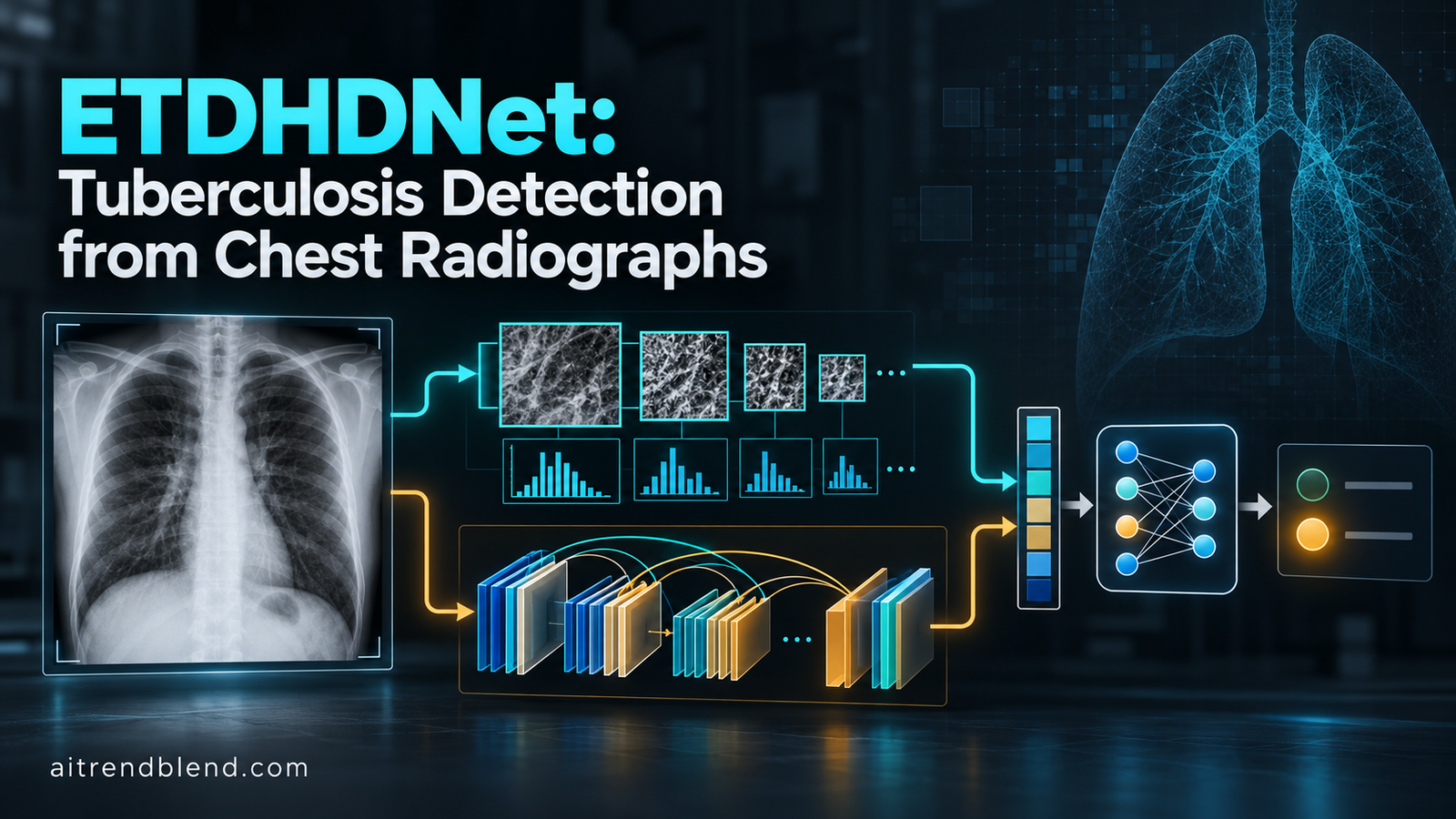
A radiologist in a district hospital reads sixty chest radiographs before lunch. Somewhere in that stack is a faint patch of haze near an upper lobe, the kind of shadow that could be old scarring, a passing infection, or early tuberculosis. The WHO figures cited in the paper say tuberculosis killed 1.25 million people in 2023 and made about 10.8 million people ill. Software that reads radiographs could stretch scarce specialist time, but only if it notices what a tired human eye can miss. A team from The University of Western Australia and King Khalid University thinks part of the answer is an old idea called texture.
Please read. This article explains published research. It is not medical advice, diagnosis, or treatment, and nothing here should guide a decision about anyone’s health. Anyone concerned about tuberculosis should speak with a qualified health professional.
Why a strong image model can still miss tuberculosis
Convolutional networks learn in layers. Early layers pick up edges and tiny patterns, later layers combine them into shapes and objects. Between those layers sit pooling operations that shrink the image so deeper layers can see wider regions. It is an efficient design and it works remarkably well on photographs of cats and cars. A chest radiograph is a different kind of picture.
Tuberculosis rarely announces itself with a clean outline. It appears as patchy opacities, clusters of small lesions, nodules, and fibrotic streaks, often with edges that fade into healthy lung. Shati, Datta, Mansoor, and Hassan argue that these cues live in fine grained intensity patterns and that repeated pooling can wash them out. Their paper, published in Intelligence Based Medicine and available as an open access article with the DOI 10.1016/j.ibmed.2025.100269, says it plainly when it notes that subtle texture cues can be overlooked in standard CNN pipelines because of detail lost during pooling.
“…subtle texture cues … can be overlooked in standard CNN pipelines due to the loss of detail from pooling operations.”
Shati et al., Intelligence Based Medicine, 2025
Here is where it gets interesting. Texture analysis is older than deep learning by decades. The Local Binary Pattern, or LBP, was built to describe how pixel intensities vary around a point, and it has been used for faces, objects, and medical images. Its weakness is scale. One LBP window sees a tiny patch, while tuberculosis lesions range from small specks to large consolidations. So the question the authors ask is whether a texture signal can be kept at several scales while a deep network supplies the global structure. Neither half has to do the whole job.
That framing matters because it is a design choice rather than a bigger network. The authors trained everything on a single NVIDIA Tesla T4 GPU in Google Colab, and they report inference times of a millisecond or two. A screening tool meant for clinics with modest hardware has to look roughly like that. For readers following the broader push toward small models that still perform, our coverage of model compression and efficient deployment goes deeper on the tradeoffs.
There is also a quieter problem the paper only touches. Models that look superb on one collection often stumble on another. Sathitratanacheewin and colleagues trained a deep convolutional network on the Shenzhen dataset and measured an AUC of 0.8502 there, then watched it fall to 0.7054 on ChestXray8, a general purpose collection that is not specific to tuberculosis. Any new TB model deserves to be read with that cautionary result in mind.
What earlier tuberculosis detectors achieved
The literature the authors review is a mix of classical machine learning and deep learning, and the reported numbers swing widely. Hooda and colleagues combined AlexNet, GoogLeNet, and ResNet in an ensemble and reached 88.24 percent accuracy and an AUC of 0.93 on a pooled set drawn from the Montgomery County, Shenzhen, Belarus, and JSRT collections. Munadi and colleagues tried image enhancement on a pretrained network and found that unsharp masking gave the best result, with 89.92 percent accuracy and an AUC of 94.8 percent on the Shenzhen data. Singh and colleagues extracted the lungs with log Gabor filtering and morphological steps, computed texture and shape features, and fed them to a support vector machine. Their AUC was 0.98 on Montgomery County and 0.96 on Shenzhen.
Kaur and Sharma took a different route and compared decision trees, naive Bayes, and support vector machines on clinical data and radiographs from hospitals in India. A decision tree reached 95 percent accuracy for both pulmonary and extra pulmonary TB. Those two classes are not the same problem as telling healthy from TB on a radiograph, so the number is hard to compare with the others.
The closest relative of ETDHDNet is the work of Fati and colleagues. They built a hybrid that extracts deep features from two CNN models and combines them with handcrafted descriptors, namely the Discrete Wavelet Transform, Grey Level Co occurrence Matrix, and LBP, before an artificial neural network makes the call. They report 99.2 percent accuracy on the Shenzhen dataset and 99.8 percent on the TB Chest Radiography Database. Hold onto that detail. We will return to it when we look at how ETDHDNet compares, because the Shenzhen number for ETDHDNet is far lower and the comparison tables in the paper do not list this earlier hybrid.
All of this sets the scene for where ETDHDNet claims its value. The authors want a model that is lighter than ensembles, needs no lung segmentation, and still carries texture information at more than one scale. For readers who like to see how texture and attention ideas meet in imaging, our notes on vision transformers and attention offer a useful contrast, because transformers chase global context while this paper chases local detail.
How ETDHDNet is built
The pipeline is short. Every radiograph is resized to 224 by 224 pixels and scaled to the range 0 to 1. That is all. There is no lung segmentation and no contrast enhancement, and the authors present this as a feature because it removes steps that can break when a model meets images from a new hospital. The processed image then travels down two parallel paths.
Path one, the ETDH texture module
The first path is the Extended Texture Descriptor Histogram. For each pixel, the module looks at a ring of neighbours at a chosen radius and asks a simple question about each one. Is it at least as bright as the centre pixel. The answers become a string of ones and zeros, which is read as a number. That is the classic LBP code. The extension is that the module does this three times with growing rings.
At radius 1 it samples 8 points around a 3 by 3 neighbourhood, which captures fine grained texture. At radius 2 it samples 16 points over a 5 by 5 region for medium patterns. At radius 3 it samples 24 points over a 7 by 7 region for coarse structure. The number of points follows a simple rule.
Each pixel’s code comes from comparing the centre intensity \(g_c\) with each neighbour \(g_n\) on the ring.
Rather than keep every possible code, the authors use uniform patterns. These are codes with at most two transitions between zeros and ones around the ring, which tend to correspond to edges, corners, and spots. All remaining codes share a pair of extra bins. That gives 10 bins at the first scale, 18 at the second, and 26 at the third. Joined together they make a 54 value vector.
Think about what this vector actually is. It is not a picture of the lungs. It is a compact summary of how often each kind of local pattern appears across the whole image, at three granularities. Position is thrown away, which is both the strength and the cost. The summary is cheap and stable, yet it cannot say where in the lung a suspicious pattern sits.
Path two, DenseNet121
The second path is a pretrained DenseNet121. Its densely connected layers pass earlier feature maps forward into later ones, which reuses features and keeps the parameter count modest. After four dense blocks the network produces a 1024 value vector that describes the image in high level terms. DenseNet121 learns shapes, regions, and relationships that no histogram can express.
Fusion and classification
The two vectors are placed side by side to form a single input of 1078 values.
A feed forward network with two dense layers of 256 neurons each, ReLU activations, and dropout reads this vector. The last layer uses a sigmoid for binary prediction and a softmax for the three class problem.
Training used the Adam optimizer for up to 100 epochs with a batch size of 16. Binary Crossentropy handled the two class tasks and Categorical Crossentropy handled the three class task.
Early stopping with a patience of 5 epochs halted training when validation performance stopped improving. The paper does not state the learning rate, the dropout rate, or whether ImageNet normalisation was applied before the backbone. Anyone trying to reproduce the work will have to pick those values, and our reference code below marks each of them as an assumption.
Key takeaway
The design philosophy is division of labour. A fixed, handcrafted histogram carries fine detail that pooling would blur, and a pretrained DenseNet121 carries structure and context. The classifier sees both at once and learns how much to trust each.
Data and experimental setup
The study uses three public collections. The first, TBX11K, holds 11,200 radiographs at 512 by 512 pixels. It was assembled from four smaller sources, including the Montgomery County and Shenzhen sets, and its three labelled folders contain 3,800 healthy cases, 3,800 sick cases without TB, and 800 TB cases. Another set of more than 3,000 images was reserved for an online competition. The second collection, which we will call DB2, comes from a team at Qatar University and the University of Dhaka with collaborators in Malaysia and at Hamad Medical Corporation. It has 3,500 healthy radiographs and 700 TB radiographs. The third is the Shenzhen dataset, created by the U.S. National Library of Medicine with Guangdong Medical College, with 662 radiographs of which 336 show TB and 326 are normal. Its TB cases include pediatric images.
The authors split every dataset at random into 70 percent for training, 10 percent for validation, and 20 percent for testing. Evaluation relied on accuracy, precision, recall, F1 score, and AUC, along with confusion matrices.
The confusion matrices let us check one detail. The three class TBX11K matrix adds up to 1,680 test images, which is exactly 20 percent of 8,400, the number of labelled healthy, sick, and TB images. So the competition images were not part of the test set. The DB2 matrix totals 840 images, which is 20 percent of 4,200, and the Shenzhen matrix totals 133, which is about 20 percent of 662. That last number matters a great deal, as we will see in the limitations.
What the results show
The headline numbers are strong on two of the three datasets. The table below reproduces the authors’ main results.
| Dataset and task | Accuracy | Precision | Recall | F1 score | AUC |
|---|---|---|---|---|---|
| TBX11K, healthy, TB, and non TB | 97.50 | 97.29 | 97.32 | 97.30 | 0.993 |
| TBX11K, TB versus non TB | 98.26 | 98.03 | 98.11 | 98.02 | 0.987 |
| TBX11K, healthy versus TB | 99.05 | 99.53 | 99.30 | 99.01 | 0.998 |
| DB2, healthy versus TB | 99.29 | 99.25 | 98.37 | 99.30 | 0.997 |
| Shenzhen, healthy versus TB | 88.05 | 88.31 | 88.14 | 88.23 | 0.930 |
Healthy versus TB on TBX11K is the easy case, since the model only has to separate clearly normal lungs from TB. Separating TB from other sick lungs is harder, and the three class task is hardest because it adds the possibility of confusing all three. The accuracy ordering follows that logic, falling from 99.05 to 98.26 to 97.50.
The Shenzhen result is the odd one out. Accuracy drops to 88.05 percent and AUC to 0.930. The authors attribute this to more complex and varied patterns, differences in image quality, and subtler features. That is plausible. It is also a reminder that the same architecture can swing by eleven points depending on the dataset, which says something about how fragile any single number is.
Does the texture module really help
The most convincing experiment in the paper is simple. The authors added the ETDH module to other backbones and measured what changed. The table below shows accuracy with and without it.
| Task | InceptionV3 | InceptionV3 with ETDH | MobileNetV2 | MobileNetV2 with ETDH | DenseNet121 | ETDHDNet |
|---|---|---|---|---|---|---|
| TBX11K three class | 91.07 | 94.17 | 94.58 | 96.49 | 95.35 | 97.50 |
| TBX11K healthy versus TB | 96.30 | 96.74 | 96.95 | 98.80 | 96.84 | 99.05 |
| TBX11K TB versus non TB | 92.82 | 94.57 | 95.54 | 96.74 | 95.86 | 98.26 |
| DB2 healthy versus TB | 97.45 | 98.62 | 99.15 | 99.28 | 98.80 | 99.29 |
| Shenzhen healthy versus TB | 84.21 | 86.46 | 85.71 | 87.90 | 85.72 | 88.05 |
The pattern is consistent. In all fifteen pairings the texture module raises accuracy. The gains are largest on the harder tasks and smallest on DB2, where baselines already sit near the ceiling. InceptionV3 on the three class task climbs from 91.07 to 94.17, a gain of 3.10 points. DenseNet121 gains 2.15 points on the same task, 2.21 on healthy versus TB, and 2.40 on TB versus non TB. On DB2 the gain is only 0.49 points, and MobileNetV2 with ETDH, at 99.28, is practically tied with the full model at 99.29.
The consistency across three different backbones is the best evidence that the texture histogram contributes something real, rather than that DenseNet121 was simply a lucky pairing.
Key takeaway
The cheapest piece of the system, a 54 value histogram that needs no training, produces gains of two to three points on harder tasks across several backbones. That is a useful lesson for anyone building medical imaging pipelines. A fixed handcrafted feature can still earn its place beside a deep network.
How many scales are enough
Tables 11 and 12 in the paper vary the number of scales. With one scale, three class accuracy is 96.31 percent. Two scales raise it to 96.67 and all three reach 97.50. On Shenzhen the climb runs from 85.71 to 86.46 to 88.05. On the easy healthy versus TB task the improvements shrink to a few hundredths of a point, from 98.91 to 98.99 to 99.05. Multiscale helps most where the problem is difficult, which fits the original motivation. The texture module on its own is weak, though. On Shenzhen, ETDH alone scores 72.02 percent and DenseNet121 alone scores 85.72, so the two parts are clearly complementary rather than interchangeable.
Speed and training behaviour
Computation time looks encouraging. Training on TBX11K took 249.26 seconds for the binary task and 452.13 seconds for the three class task. DB2 took 234.07 seconds and Shenzhen 89.01 seconds. Inference figures in the table are listed as 0.0007 to 0.002, and the text describes them as milliseconds, although the table heading says seconds. The paper does not say whether the numbers are per image, so treat them as a rough sign of lightness rather than a benchmark. Training and validation losses stay close on the large datasets, for example 0.0443 and 0.0576 on the three class task. On Shenzhen they are higher, at 0.2472 and 0.2663.
Reading the numbers with a sceptical eye
None of what follows is meant as an attack on the work. It is the sort of reading any careful reviewer would do, and the authors would probably welcome it.
A few numbers that do not quite agree
The first is small. Our arithmetic from the three class confusion matrix gives 753 plus 745 plus 137 correct out of 1,680, or 97.32 percent. That matches the reported recall of 97.32 but not the reported accuracy of 97.50. The healthy versus TB matrix gives 99.02 percent against a reported 99.05, and the Shenzhen matrix gives 87.97 percent against 88.05. Differences like these could come from averaging over several runs or from rounding, and the paper does not say which. They are tiny, yet they leave the reader unsure which figure came from which run.
The second is larger. The discussion states that on the Shenzhen set ETDHDNet beats DenseNet121 by 2.78 points and ETDH by 16.48 points. The tables show 88.05 against 85.72 and 72.02, which are gaps of 2.33 and 16.03 points. The tables and the text should agree, and a reader citing this paper should quote the table values.
The weak spot inside the three class result
Look at the three class confusion matrix. Of 163 true TB cases, 137 were correct, 20 were labelled sick but not TB, and 6 were labelled healthy. That is a TB recall of about 84 percent, far below the 97 percent overall figure. Overall accuracy looks excellent because the healthy and non TB groups are about 4.6 times larger than the TB group, and the model handles them well. In the binary healthy versus TB task the model finds 156 of 162 TB cases, or roughly 96 percent. A screening tool is judged by its misses. The authors acknowledge slightly higher false negatives in TB detection, and the matrices suggest that confusion with other lung disease is the main driver.
Comparisons across papers need care
The paper compares itself with published methods in three tables. The table below picks out representative rows.
| Dataset | Method | Accuracy | AUC |
|---|---|---|---|
| TBX11K three class | Faster R CNN with ResNet50 and FPN | 89.7 | 0.936 |
| TBX11K three class | SSD with VGG Net16 | 88.2 | 0.938 |
| TBX11K three class | SymFormer with RetinaNet | 94.6 | 0.991 |
| TBX11K three class | ETDHDNet | 97.50 | 0.993 |
| DB2 healthy versus TB | DenseNet201 | 98.60 | not listed |
| DB2 healthy versus TB | EfficientNetB0 and ResNet50 | 98.20 | not listed |
| DB2 healthy versus TB | ETDHDNet | 99.29 | 0.997 |
| Shenzhen | MobileNet | 90.2 | not listed |
| Shenzhen | EfficientNet with enhancement | 89.92 | 0.948 |
| Shenzhen | ETDHDNet | 88.05 | 0.930 |
Three cautions apply. First, the TBX11K rivals in the three class table are detection models that locate TB regions as well as classify, so they solve a harder problem than a pure classifier. Their accuracy and AUC may not be measured the same way. Second, every study used its own split, and in some cases its own preprocessing, so the numbers are not from a shared test bench. Third, on Shenzhen ETDHDNet does not lead. MobileNet and an EfficientNet pipeline both post higher accuracy, and the authors say so. The earlier hybrid by Fati and colleagues, described in the introduction with 99.2 percent on Shenzhen, is absent from the tables altogether. We cannot tell whether the two were evaluated under comparable conditions, but a reader deserves to see them side by side.
Key takeaway
The cleanest claim in this paper is relative rather than absolute. Adding the texture module to several backbones helps every time. The claim to be most careful with is the leaderboard one, since splits, tasks, and metrics differ from study to study.
Where a lab result and a hospital part ways
Clinical translation gap
A model scoring 99 percent on a curated public dataset has cleared the first hurdle, and only the first. Several gaps remain between that result and a clinic.
The first is prevalence. In the TBX11K labelled data, TB cases make up 800 of 8,400 images, about 9.5 percent. DB2 holds 700 of 4,200, about 16.7 percent, and Shenzhen holds 336 of 662, about 51 percent. A real screening programme usually sees far fewer positives. That matters because the share of positive calls that are truly TB falls sharply as the condition becomes rarer. As an illustration only, using the healthy versus TB matrix (sensitivity near 96.3 percent and specificity near 99.6 percent) and assuming TB in one percent of screened people, roughly 71 percent of positive calls would be correct. That calculation ignores every other lung disease a real clinic sees, so the true figure could be lower.
The second is who is in the image. The authors note that their public datasets come from specific institutions and, in the Shenzhen case, include pediatric images. Scanner type, exposure settings, patient age, and local disease patterns all shift the pixel statistics that a texture histogram reads. Because LBP is built on raw intensity comparisons, it may be sensitive to differences in how images are produced. The paper does not test that.
The third is what the output is for. A classifier that returns a probability is not a diagnosis. It could prioritise a worklist, flag a case for a second read, or support a community screening drive. Each use has its own acceptable error rate, and the cost of a missed case is very different from the cost of an extra confirmatory test.
Regulatory and safety notes
Software that influences diagnosis is generally treated as a medical device in many jurisdictions. Moving from this research prototype to clinical use would normally require a defined intended use, prospective validation on local patients, bias and subgroup analysis, human oversight, and monitoring after deployment. The authors are explicit that further validation and clinical trials are needed, and they list domain generalisation as future work. We agree with that assessment and would add that evidence from peer reviewed prospective studies, rather than from a single retrospective split, should carry the most weight for any clinical claim.
Clinical limitations the paper leaves open
Sample size. The Shenzhen test set holds roughly 133 images. A single misclassified image shifts accuracy by about 0.75 points, and the model made 16 errors on that set. A gap of one or two points between methods on this dataset, such as the gap to MobileNet or EfficientNet, sits well inside what a different random split could produce. The paper reports no confidence intervals and no significance tests. Even the larger TBX11K test set has only 163 TB cases in the three class matrix.
Dataset bias. TBX11K is stitched together from four smaller sources. DB2 draws on several collections. Shenzhen is a single hospital programme. Models can learn shortcuts such as the acquisition style of a source rather than the disease. Splits were random, and the paper does not say whether they were made at patient level. If one person contributed several images, near duplicates could land in both training and test sets.
Generalisation. Every result comes from training and testing within the same dataset. The authors state that cross domain evaluation on unseen collections is future work. Given the earlier finding that an AUC of 0.8502 fell to 0.7054 on an unrelated collection, this is the single most important missing experiment.
Interpretability. The model mixes handcrafted histograms with deep features, which is hard to explain with gradient based saliency maps because those tools only reach the convolutional part. The authors plan to try model agnostic methods such as SHAP and LIME. Until then, a clinician cannot see which texture pattern or lung region drove a prediction.
Task scope. The model separates healthy, sick without TB, and TB. It was not built to grade severity, locate lesions, or handle cases where TB sits alongside other disease. The authors mention possible extension to CT, COVID, and pneumonia, though none of that is tested here.
Conclusion
ETDHDNet delivers a modest, believable result. On the two larger datasets it reaches accuracy between 97.50 and 99.29 percent, and on the harder Shenzhen set it reaches 88.05 percent with an AUC of 0.930. The sturdiest finding is the ablation. Across three backbones and five tasks, adding a 54 value texture histogram raised accuracy every time, usually by two to three points on harder problems.
The conceptual shift is small but healthy. For years the story in medical imaging has been that deep networks learn everything and handcrafted features are obsolete. This paper offers a gentler position. Pooling throws away information, and a cheap fixed descriptor can put some of it back. The right question is not which camp wins but which signal the network is least likely to learn on its own.
The idea should travel. Any imaging task where the evidence sits in fine grained surface patterns could borrow it. Skin lesions, retinal images, histology slides, and industrial surface inspection all come to mind. The authors suggest extending the approach to other respiratory diseases and to CT. A multiscale LBP histogram costs almost nothing to compute, so testing it beside a modern backbone is a cheap experiment for any team.
The limitations are real. Every number comes from a random split of public data. There are no confidence intervals, no external validation, and a few small mismatches between tables and text. The three class TB recall of about 84 percent is a warning against reading 97.50 percent as clinical readiness. Comparisons with earlier work mix tasks and protocols, and the Shenzhen result shows how quickly a headline number can shrink. A reader should treat this paper as a promising component study rather than evidence of a deployable screening tool.
The next steps are clear from the paper itself. Test on unseen institutions, scanners, and populations. Report intervals over repeated runs. Add explanations that cover the handcrafted branch. Explore whether shape aware and context aware features can add what a histogram cannot, such as location. If those tests hold up, a lightweight model like this could earn a place in the screening queue.
The honest summary is that texture was not forgotten, only sidelined, and it still has something to say about a lung.
Reference implementation in PyTorch
The code below is an independent reconstruction written from the paper’s description, so it may differ from the authors’ own implementation. It includes the multiscale ETDH module, the DenseNet121 branch, the fused classifier, both loss functions, a training loop with early stopping, an evaluation function, and a smoke test on dummy data. Values the paper does not give, such as the learning rate and dropout rate, are marked as assumptions in the comments. Set pretrained=True for real experiments.
"""
ETDHDNet reference implementation (PyTorch).

Independent re-implementation written from the description in
Shati et al., Intelligence Based Medicine 12 (2025) 100269.
Values the paper does not state (learning rate, dropout rate, ImageNet
normalisation) are marked ASSUMPTION and are choices made here, not the authors'.
"""
import math
import time
import numpy as np
import torch
import torch.nn as nn
import torch.nn.functional as F
from torch.utils.data import DataLoader, TensorDataset
from torchvision import models


# ----------------------------------------------------------------------------
# 1. ETDH module: multiscale uniform LBP histograms (radii 1, 2, 3 and points 8r)
# ----------------------------------------------------------------------------
class ETDH(nn.Module):
    """Extended Texture Descriptor Histogram.

    For every scale s with radius r, p = 8 * r neighbours are sampled on a circle
    around each pixel (bilinear interpolation). Each neighbour is compared with
    the centre pixel, the bits form an LBP code, and the code is mapped to the
    rotation invariant uniform pattern set with p + 2 bins. With radii 1, 2, 3
    this gives 10 + 18 + 26 = 54 bins, concatenated into FV_ETDH.
    """

    def __init__(self, radii=(1, 2, 3)):
        super().__init__()
        self.radii = tuple(radii)
        self.points = tuple(8 * r for r in radii)          # Eq. (1)
        self.out_dim = sum(p + 2 for p in self.points)      # 54 for the default

    @staticmethod
    def _neighbour_offsets(p, r):
        k = np.arange(p)
        ang = 2.0 * math.pi * k / p
        dy = np.round(-r * np.sin(ang), 6)
        dx = np.round(r * np.cos(ang), 6)
        return dy, dx

    @torch.no_grad()
    def _lbp_bins(self, gray, p, r):
        """gray is (B, 1, H, W). Returns an integer map (B, H, W) of bin indices."""
        _, _, h, w = gray.shape
        pad = r + 1
        xp = F.pad(gray, (pad, pad, pad, pad), mode="replicate")
        centre = gray[:, 0]
        dy, dx = self._neighbour_offsets(p, r)

        def crop(oy, ox):
            return xp[:, 0, pad + oy: pad + oy + h, pad + ox: pad + ox + w]

        bits = []
        for k in range(p):
            y0, x0 = int(math.floor(dy[k])), int(math.floor(dx[k]))
            fy, fx = float(dy[k] - y0), float(dx[k] - x0)
            val = (
                (1 - fy) * (1 - fx) * crop(y0, x0)
                + (1 - fy) * fx * crop(y0, x0 + 1)
                + fy * (1 - fx) * crop(y0 + 1, x0)
                + fy * fx * crop(y0 + 1, x0 + 1)
            )
            bits.append((val >= centre).to(torch.int16))
        bits = torch.stack(bits, dim=1)                      # (B, p, H, W)
        ones = bits.sum(dim=1)                               # number of 1 bits
        transitions = (bits != torch.roll(bits, 1, dims=1)).sum(dim=1)
        # uniform patterns (at most 2 transitions) use their count of ones (0..p)
        # every other pattern shares the last bin (p + 1)
        return torch.where(transitions <= 2, ones, torch.full_like(ones, p + 1)).long()

    @torch.no_grad()
    def forward(self, gray):
        batch = gray.shape[0]
        hists = []
        for p, r in zip(self.points, self.radii):
            bins = self._lbp_bins(gray, p, r).reshape(batch, -1)
            hist = torch.zeros(batch, p + 2, device=gray.device)
            hist.scatter_add_(1, bins, torch.ones_like(bins, dtype=torch.float32))
            hists.append(hist / bins.shape[1])               # normalised H(s_i)
        return torch.cat(hists, dim=1)                       # FV_ETDH, Eq. (2)


# ----------------------------------------------------------------------------
# 2. DenseNet121 branch (hierarchical feature learning, 1024 dimensional output)
# ----------------------------------------------------------------------------
class DenseNetBranch(nn.Module):
    def __init__(self, pretrained=True):
        super().__init__()
        weights = models.DenseNet121_Weights.DEFAULT if pretrained else None
        self.features = models.densenet121(weights=weights).features
        # ASSUMPTION: ImageNet statistics for the pretrained backbone
        self.register_buffer("mean", torch.tensor([0.485, 0.456, 0.406]).view(1, 3, 1, 1))
        self.register_buffer("std", torch.tensor([0.229, 0.224, 0.225]).view(1, 3, 1, 1))
        self.out_dim = 1024

    def forward(self, x):
        x = (x - self.mean) / self.std
        f = F.relu(self.features(x), inplace=False)
        return F.adaptive_avg_pool2d(f, 1).flatten(1)       # FV_D, Eq. (3)


# ----------------------------------------------------------------------------
# 3. Full model: concatenation (1078 dims) and feed forward MLP head
# ----------------------------------------------------------------------------
class ETDHDNet(nn.Module):
    """num_classes = 1 for binary prediction (sigmoid), 3 for Healthy, TB, Non TB."""

    def __init__(self, num_classes=1, pretrained=True, hidden=256, dropout=0.3):
        super().__init__()
        self.etdh = ETDH()
        self.dense = DenseNetBranch(pretrained)
        fused_dim = self.etdh.out_dim + self.dense.out_dim   # 54 + 1024 = 1078
        self.head = nn.Sequential(
            nn.Linear(fused_dim, hidden), nn.ReLU(inplace=True), nn.Dropout(dropout),
            nn.Linear(hidden, hidden), nn.ReLU(inplace=True), nn.Dropout(dropout),
            nn.Linear(hidden, num_classes),
        )
        self.num_classes = num_classes

    def forward(self, x):
        """x is (B, 3, 224, 224) scaled to [0, 1]. Returns logits."""
        gray = x.mean(dim=1, keepdim=True)
        fv_etdh = self.etdh(gray)
        fv_d = self.dense(x)
        fused = torch.cat([fv_etdh, fv_d], dim=1)            # Eq. (4)
        return self.head(fused)

    @torch.no_grad()
    def predict_proba(self, x):
        logits = self.forward(x)
        if self.num_classes == 1:
            return torch.sigmoid(logits).squeeze(1)          # Eq. (5)
        return torch.softmax(logits, dim=1)                  # Eq. (6)


# ----------------------------------------------------------------------------
# 4. Losses that match the paper
# ----------------------------------------------------------------------------
def binary_cross_entropy_loss(logits, targets):
    return F.binary_cross_entropy_with_logits(logits.squeeze(1), targets.float())


def categorical_cross_entropy_loss(logits, targets):
    return F.cross_entropy(logits, targets.long())


def make_loss(num_classes):
    return binary_cross_entropy_loss if num_classes == 1 else categorical_cross_entropy_loss


# ----------------------------------------------------------------------------
# 5. Evaluation
# ----------------------------------------------------------------------------
@torch.no_grad()
def evaluate(model, loader, device="cpu"):
    from sklearn.metrics import (accuracy_score, precision_recall_fscore_support,
                                 roc_auc_score, confusion_matrix)
    model.eval()
    loss_fn = make_loss(model.num_classes)
    total_loss, n, probs, labels = 0.0, 0, [], []
    for xb, yb in loader:
        xb, yb = xb.to(device), yb.to(device)
        logits = model(xb)
        total_loss += loss_fn(logits, yb).item() * xb.size(0)
        n += xb.size(0)
        if model.num_classes == 1:
            probs.append(torch.sigmoid(logits).squeeze(1).cpu())
        else:
            probs.append(torch.softmax(logits, dim=1).cpu())
        labels.append(yb.cpu())
    probs, labels = torch.cat(probs).numpy(), torch.cat(labels).numpy()
    if model.num_classes == 1:
        pred = (probs >= 0.5).astype(int)
        auc = roc_auc_score(labels, probs) if len(np.unique(labels)) > 1 else float("nan")
        avg = "binary"
    else:
        pred = probs.argmax(1)
        try:
            auc = roc_auc_score(labels, probs, multi_class="ovr")
        except ValueError:
            auc = float("nan")
        avg = "weighted"
    pre, rec, f1, _ = precision_recall_fscore_support(labels, pred, average=avg, zero_division=0)
    return {
        "loss": total_loss / max(n, 1),
        "acc": accuracy_score(labels, pred),
        "precision": pre, "recall": rec, "f1": f1, "auc": auc,
        "confusion": confusion_matrix(labels, pred),
    }


# ----------------------------------------------------------------------------
# 6. Training loop (Adam, early stopping with patience 5, up to 100 epochs)
# ----------------------------------------------------------------------------
def train(model, train_loader, val_loader, epochs=100, lr=1e-4, patience=5, device="cpu"):
    # ASSUMPTION: lr = 1e-4. The paper names Adam but not the learning rate.
    model.to(device)
    loss_fn = make_loss(model.num_classes)
    opt = torch.optim.Adam([p for p in model.parameters() if p.requires_grad], lr=lr)
    best, best_state, bad = float("inf"), None, 0
    for epoch in range(1, epochs + 1):
        model.train()
        t0, running = time.time(), 0.0
        for xb, yb in train_loader:
            xb, yb = xb.to(device), yb.to(device)
            opt.zero_grad()
            loss = loss_fn(model(xb), yb)
            loss.backward()
            opt.step()
            running += loss.item() * xb.size(0)
        val = evaluate(model, val_loader, device)
        print(f"epoch {epoch:03d} train_loss {running / len(train_loader.dataset):.4f} "
              f"val_loss {val['loss']:.4f} val_acc {val['acc']:.4f} ({time.time() - t0:.1f}s)")
        if val["loss"] < best - 1e-5:
            best, bad = val["loss"], 0
            best_state = {k: v.detach().clone() for k, v in model.state_dict().items()}
        else:
            bad += 1
            if bad >= patience:
                print("early stopping")
                break
    if best_state is not None:
        model.load_state_dict(best_state)
    return model


# ----------------------------------------------------------------------------
# 7. Smoke test on dummy data (no download, no GPU needed)
# ----------------------------------------------------------------------------
def _dummy_loader(n, num_classes, size=96, batch=8, seed=0):
    g = torch.Generator().manual_seed(seed)
    x = torch.rand(n, 3, size, size, generator=g)
    if num_classes == 1:
        y = torch.randint(0, 2, (n,), generator=g)
    else:
        y = torch.randint(0, num_classes, (n,), generator=g)
    return DataLoader(TensorDataset(x, y), batch_size=batch, shuffle=True)


if __name__ == "__main__":
    torch.manual_seed(0)
    # the ETDH vector must have 54 entries and each histogram must sum to one
    probe = ETDH()(torch.rand(2, 1, 64, 64))
    assert probe.shape == (2, 54), probe.shape
    assert torch.allclose(probe[:, :10].sum(1), torch.ones(2)), "scale 1 histogram"

    for k in (1, 3):                                         # binary, then three class
        model = ETDHDNet(num_classes=k, pretrained=False)    # pretrained=True for real use
        tr, va = _dummy_loader(32, k), _dummy_loader(16, k, seed=1)
        logits = model(next(iter(tr))[0])
        assert logits.shape == (8, k), logits.shape
        train(model, tr, va, epochs=2, patience=5)
        print("metrics", {m: v for m, v in evaluate(model, va).items() if m != "confusion"})
    print("smoke test passed")
Frequently asked questions
What is ETDHDNet?
ETDHDNet is a tuberculosis prediction model for chest radiographs. It joins a 54 value multiscale texture histogram with the 1024 value feature vector from a pretrained DenseNet121, then classifies the combined 1078 values with a small feed forward network.
How accurate is ETDHDNet at detecting tuberculosis?
The authors report 99.05 percent accuracy for healthy versus TB and 97.50 percent for three class prediction on TBX11K, 99.29 percent on a second database, and 88.05 percent on the Shenzhen dataset. These come from random splits of public data, so they are not a measure of real clinic performance.
Why combine texture features with DenseNet121?
Pooling inside a convolutional network can blur fine intensity patterns such as small opacities and fibrotic streaks. A local binary pattern histogram keeps that detail at three scales, while DenseNet121 supplies shape and context. In the paper, adding the texture module raised accuracy for every backbone tested.
Can ETDHDNet diagnose tuberculosis in a patient?
No. It is a research model tested on public datasets, with no prospective study or clinical trial. Diagnosis needs a qualified health professional, and any real deployment would need local validation and regulatory review.
Which datasets did the study use and are they public?
The study used TBX11K with 11,200 radiographs, a database from Qatar University and the University of Dhaka with 3,500 healthy and 700 TB images, and the Shenzhen dataset with 662 images. The authors describe all three as open access.
What are the main limitations of the study?
Each result comes from one random split of one dataset at a time. There are no confidence intervals, no cross dataset testing, and a small Shenzhen test set of about 133 images. Three class TB recall computed from the confusion matrix is about 84 percent, and the handcrafted branch is not yet explained by any interpretability method.
Read the original study
The full paper is open access, and the TBX11K dataset used in the largest experiments is available from Kaggle.
Shati, A., Datta, A., Mansoor, A., and Hassan, G. M. (2025). ETDHDNet: An advanced DenseNet-based extended texture descriptor for efficient tuberculosis prediction in CXR images. Intelligence-Based Medicine, 12, 100269. https://doi.org/10.1016/j.ibmed.2025.100269
This analysis is based on the published paper and an independent evaluation of its claims.
Related reading on aitrendblend
For wider context, see our hub for AI in medical imaging and healthcare.