
- Test time adaptation
- Domain generalization
- Distribution shift
- Contrastive learning
- Prototypes
- Gaussian mixture model
- Image classification
- PyTorch
Imagine a camera trap strapped to a tree in a forest the model has never seen. The classifier inside it was trained on photos from three other locations, and it learned them well. Here the light falls differently, the undergrowth is a different green, and the animals sit in unfamiliar poses. Accuracy slips. Nobody can send labelled images from this exact spot, and nobody wants to retrain a network for every hillside. Yet the photos keep arriving, thousands of them, unlabelled but free. Saeed Karimi and Hamdi Dibeklioğlu at Bilkent University ask a pointed question about that stream. Can the model teach itself something useful while it works, without being led astray by its own mistakes?
Key points
- AdaPAC adapts a trained image classifier during inference using unlabeled test batches. Before deployment it clusters source features inside each class into sub class prototypes.
- At test time a Gaussian mixture over those clusters splits every batch into reliable and unreliable samples. Reliable ones get a prototypical contrastive loss, unreliable ones are contrasted with nearby reliable samples, and a gradient similarity score damps risky layers.
- With ResNet-50 it reaches 71.5% average accuracy on four benchmarks against 68.3% for plain ERM, with gains of 1.4, 5.1, 2.7 and 3.7 points on VLCS, PACS, OfficeHome and TerraIncognita.
- It is not the best method on VLCS, where eleven other rows in the paper’s ResNet-50 comparison score higher than its 77.6%.
- Other tables suggest gains shrink as the starting model gets stronger, and that several hundred test samples are needed before the benefit shows.
- The paper reports GPU memory but no timing, and it never tests hostile or drifting test streams.
Why adapting at test time is tempting, and risky
Domain generalization asks a model to cope with data from a domain it never saw in training. The usual recipe is to train on several source domains and hope the learned features carry over. The authors point to a study by Gulrajani and Lopez-Paz which found that many such methods fail to improve much on plain empirical risk minimization, usually shortened to ERM. If extra training tricks do not help much, perhaps the unlabeled test images themselves hold the missing information.
That is the idea behind test time adaptation, or TTA. The model updates its own weights as batches of unlabeled test data stream in. Tent, a well known method, minimizes the entropy of the model’s predictions and updates only batch normalization parameters. T3A skips gradient descent altogether and adjusts only the final classifier. Others keep the high confidence predictions and train on them as if they were labels.
The trouble starts when the shift is large. The paper lists the failure modes plainly. Pseudo labels get noisier exactly when the domain gap grows, so the model reinforces its own errors. Entropy minimization pushes features away from decision boundaries and tends to pile samples onto a few dominant classes. Selection rules that keep only confident samples depend on thresholds that are fiddly to tune. And updating the whole network on noisy samples risks overfitting, while updating only a small part, such as batch norm layers or the classifier, tends to give only slight gains.
There is a quieter point about geometry. Most TTA methods pull a test feature toward a single prototype for its class. A class like dog covers cartoons, sketches, photos and everything between, so one prototype can sit far from many perfectly legitimate samples. If such a sample is misclassified, chasing the wrong prototype across a long distance can wreck the model quickly.
Readers of our Adversarial ML and AI Security coverage will recognise the shape of the problem. There is no attacker here. A model still fails because the world drifted away from its training data, and the paper never mentions adversaries. Pseudo label noise is also a familiar enemy in semi supervised work, which we saw in our piece on adapting FixMatch to marine anomaly segmentation.
How AdaPAC works
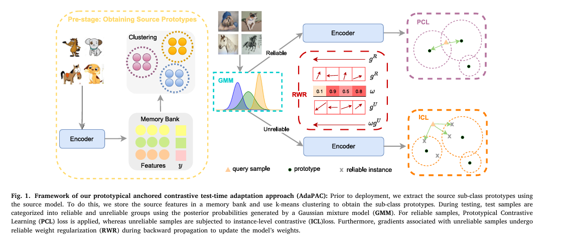
AdaPAC stands for prototypical anchored contrastive test time adaptation. The name is a mouthful, but the design follows one idea. Use the source data once, before deployment, to build a small set of anchors. Then let those anchors decide which test samples can be trusted and what they should be pulled toward.
Before deployment, learn the shape of each class
Once the source model is trained, the authors pass source data through it and store the features in a memory bank. Within each class they run k means clustering, so a class gets several sub class prototypes instead of one. The paper reports good results with 3 to 10 clusters per class. Each cluster also gets a variance and a width, which is simply the mean distance of its members to its centre.
The mean distance of the n features in cluster k of class c to its prototype. The widths are normalized across all clusters and then serve as a separate temperature for every prototype.
Needing source features at deployment time is worth a pause. AdaPAC is not source free. It keeps prototypes and variances, not the images, and the authors measure the extra memory at about 20 MB on PACS with ResNet-50. Still, a team that has thrown away its training data cannot use it.
At test time, sort the batch into trusted and untrusted
Each incoming test batch of 64 images is embedded, and a Gaussian mixture model with one isotropic component per cluster computes how likely each embedding is to belong to each cluster. If any cluster claims the sample with probability at or above a threshold, the sample counts as reliable. Otherwise it is unreliable. The authors use a threshold of 0.90 in their selection comparison and show that anything from 0.5 to 0.9 behaves about the same.
The probability that embedding z belongs to cluster k of class c. A sample is reliable when at least one cluster reaches the threshold.
“reliable samples belong to at least one cluster with high probability”Karimi and Dibeklioğlu, Neurocomputing, 2025
Reliable samples receive a prototypical contrastive loss. Each sample is pulled toward the prototypes of the clusters that claimed it and pushed away from every other prototype, with each cluster’s width setting its own temperature.
The set P holds the clusters that claim the sample. Every prototype in the bank acts as a negative for the rest.
Unreliable samples cannot be pulled toward a prototype, because they sit far from all of them and the pull could be large and misleading. Instead they are contrasted against their nearest reliable test samples, kept in a second memory bank that grows during adaptation. Those neighbours are closer than any prototype, so the loss stays gentler.
The M nearest reliable embeddings are the positives and the whole reliable memory forms the denominator. The paper reuses the letter K for neighbours as well as for clusters per class, so we write M here.
Reliable weight regularization in plain words
The last piece is the cleverest and the least intuitive. For every layer, the method computes the gradient that the reliable samples would apply and the gradient that the unreliable samples would apply. If the two point the same way, the unreliable samples are probably asking for something sensible in that layer. If they disagree, the unreliable gradient gets a smaller weight for that layer. The weight is the cosine similarity between the two gradients, rescaled across layers to run from 0 to 1.
The gradients g of the reliable and unreliable losses are compared layer by layer. After min max rescaling, the weights omega scale the unreliable gradient. The paper uses alpha both here, as a step size, and as the probability threshold in sample selection.
One consequence is easy to miss. Because of the min max rescaling, every batch has some layer that receives a weight of exactly 0 and some layer that receives exactly 1, however well or badly the gradients agree overall. The mechanism is relative, a ranking of layers, and not an absolute check on agreement. That may well be enough in practice. The paper does not test it, so we mention it as something to watch.
Two practical details help when reading the results. Algorithm 1 computes predictions first and adapts afterwards, so each batch is scored by the model as it stood before it saw that batch. That is the honest way to measure online adaptation. And batch normalization layers stay frozen while the other feature extractor parameters are updated.
What the benchmarks show
The setup
The authors test on four standard domain generalization datasets. In each run one domain is held out as the target and the other domains serve as sources.
| Dataset | Examples | Classes | Domains |
|---|---|---|---|
| VLCS | 10,729 | 5 | Caltech101, LabelMe, SUN09, VOC2007 |
| PACS | 9,991 | 7 | Art painting, cartoon, photo, sketch |
| OfficeHome | 15,588 | 65 | Artistic, clipart, product, real world |
| TerraIncognita | 24,788 | 10 | Four camera trap locations named L100, L38, L43 and L46 |
Source domains are split 80 and 20 into training and validation sets, and hyperparameters are chosen on the source validation data before any test sample is seen. Results are averaged over three runs with different seeds and splits. Source training uses Adam with a learning rate of 0.00005, and test time adaptation uses batches of 64. ResNet-50 is the main backbone, and the code builds on the public T3A library.
Headline numbers
| Method | VLCS | PACS | OfficeHome | TerraIncognita | Average |
|---|---|---|---|---|---|
| ERM | 76.2 | 83.8 | 66.8 | 46.5 | 68.3 |
| T3A | 77.8 | 84.5 | 67.9 | 46.9 | 69.3 |
| ETA | 75.9 | 85.8 | 68.4 | 48.6 | 69.7 |
| TSD | 76.5 | 88.6 | 68.4 | 44.5 | 69.5 |
| DomainAdaptor | 78.5 | 88.2 | 68.3 | 44.5 | 69.9 |
| mDSDI (trained for generalization) | 79.0 | 86.2 | 69.2 | 48.1 | 70.6 |
| AdaPAC | 77.6 | 88.9 | 69.5 | 50.2 | 71.5 |
On the average over four benchmarks AdaPAC reaches 71.5% with ResNet-50, against 68.3% for ERM. That is an average gain of 3.2 points. Per dataset the gains over ERM are 1.4 points on VLCS, 5.1 on PACS, 2.7 on OfficeHome and 3.7 on TerraIncognita.
The comparison with other methods is where the nuance lives. AdaPAC has the best average, ahead of the best generalization method, mDSDI, by 0.9 points and ahead of the best TTA rival, DomainAdaptor, by 1.6. It also has the top score on PACS, OfficeHome and TerraIncognita. It does not on VLCS. There it scores 77.6%, and eleven other rows in the paper’s ResNet-50 comparison score higher, including mDSDI at 79.0% and T3A at 77.8%, which adjusts only a classifier and takes no gradient steps. The abstract says AdaPAC outperformed the leading methods across benchmarks including VLCS. The table says otherwise, and the results text lists only the other three datasets as wins.
The margins on those three wins deserve calibration. On PACS, AdaPAC’s 88.9 ± 0.8 sits 0.3 points above TSD at 88.6 ± 1.7. On TerraIncognita its 50.2 ± 1.8 is 1.6 above ETA and SagNet at 48.6, whose spreads are 1.5 and 1.0, so the ranges overlap. With only three seeds, those spreads are rough.
There is a quieter warning in the same table. On TerraIncognita, where ERM scores 46.5%, pseudo label adaptation falls to 33.8, SHOT to 36.4, Tent to 39.5 and SAR to 38.8. Adapting on noisy samples can do real damage, which is the problem AdaPAC was built to avoid.
A small bookkeeping point. The paper’s own ERM number for PACS appears as 83.8, 83.9, 83.7 and 84.0 across its Tables 1, 2, 5 and 7, and AdaPAC with ResNet-50 on PACS appears as 88.9 in some tables and 89.1 in others. Its OfficeHome score is 69.5 in the first table and 69.3 in the fifth. Differences of two or three tenths of a point look like run to run noise, and that is the same size as AdaPAC’s 0.3 point margin over mDSDI on OfficeHome. Finally, the generalization rows come mostly from published numbers or an earlier study, while the ERM and TTA rows are the authors’ own runs. That is common practice, but it means the table mixes two sets of experimental conditions.
Which part earns its keep
| Variant | Components | Average | Gain |
|---|---|---|---|
| A | Source model only | 83.9 | None |
| B | PCL | 87.2 | 3.3 points |
| C | PCL and ICL | 88.2 | 1.0 point |
| D | PCL, ICL and RWR (AdaPAC) | 88.9 | 0.7 points |
Prototypical contrastive learning with Gaussian mixture selection delivers roughly two thirds of the total gain, 3.3 of 5.0 points. Instance contrastive learning adds 1.0 and reliable weight regularization adds 0.7. The per domain results show the regularizer’s gain is 0.7 on art painting, 1.2 on cartoon, 0.9 on sketch and nothing on photo, against standard deviations between 0.4 and 1.9. Two caveats apply. The ablation adds components in one fixed order, so we never see regularization without ICL, or ICL without PCL. And a gain below the standard deviation across three seeds is suggestive, not settled.
The paper also pits its Gaussian mixture selection against the confidence rule of PL, the entropy rule of ETA and the entropy plus gradient norm rule of SAR. Averaged over the four benchmarks, the mixture scores 70.4%, ETA 69.6%, SAR 65.6% and PL 62.9%, with the source model at 68.4%. The text says the PCL loss is applied to whichever samples each rule selects. Yet the descriptions of PL, ETA and SAR also mention their own losses, and the averages sit close to those of the full methods in the headline table, which are 62.5, 69.7 and 65.0. It is hard to tell from the paper whether this comparison isolates selection or compares whole methods.
Cluster specific temperature helps a little everywhere. Compared with a fixed temperature it adds 0.4 points on VLCS, 0.9 on PACS, 0.7 on OfficeHome and 0.6 on TerraIncognita. Sensitivity studies on PACS show the method works with 3 to 10 clusters per class and degrades at 20, with a single cluster per class clearly lower, which supports the multiple prototype idea. Small numbers of positive neighbours behave well and larger ones hurt.
Other backbones and other training methods
| Backbone | Baseline | With AdaPAC | Gain |
|---|---|---|---|
| ResNet-18 | 64.9 | 68.3 | 3.4 |
| ResNet-50 | 68.2 | 71.5 | 3.3 |
| BiT-M-R50x3 | 71.1 | 73.7 | 2.6 |
| ViT-B16 | 71.6 | 73.2 | 1.6 |
| Mixer-L16 | 67.2 | 70.0 | 2.8 |
AdaPAC improves every backbone, which is reassuring. The authors note that weaker baselines gain more, and the per dataset numbers back that up. On ViT-B16, which has the strongest OfficeHome baseline in the table at 78.5%, AdaPAC adds 0.7 points. On VLCS it adds 0.6. The ViT does gain 3.7 points on PACS, so the pattern is a tendency, not a law.
| Starting model | Before | After | Gain |
|---|---|---|---|
| ERM | 84.0 | 88.9 | 4.9 |
| RSC | 84.7 | 88.8 | 4.1 |
| CORAL | 86.1 | 89.1 | 3.0 |
| SWAD | 87.7 | 89.5 | 1.8 |
This table is the most revealing one in the paper. Before adaptation, the four models span 3.7 points. Afterwards they span 0.7. Either adaptation erases most of the advantage of better training, or PACS has a ceiling near 89 for these models. The ViT reaching 90.2 on the same dataset suggests the ceiling is soft. Either way, it hints that a strong adaptation step can stand in for some training time sophistication.
How many test samples does it need?
| Method | 64 | 128 | 256 | 512 | 1024 | 2048 |
|---|---|---|---|---|---|---|
| Tent | 84.0 | 84.0 | 84.2 | 84.5 | 85.0 | 85.4 |
| T3A | 83.8 | 83.9 | 84.1 | 84.1 | 84.3 | 84.5 |
| ETA | 83.9 | 84.0 | 84.1 | 84.4 | 84.9 | 85.6 |
| AdaPAC | 84.0 | 84.3 | 84.9 | 86.3 | 87.8 | 88.4 |
At 64 and 128 samples AdaPAC is level with its rivals and barely above the 83.9% reported for the source model. By 512 samples it leads by roughly two points, and by 2048 it reaches 88.4% against 85.6% for ETA. The protocol here adapts on a subset and then evaluates on the whole target set, which differs from the online setting of the headline table. The practical reading is simple. Hundreds of unlabeled images from the same domain have to arrive before the method pays off.
The cost side
AdaPAC is not cheap, and the authors say so. It stores prototypes, variances and a growing memory of reliable samples, which they put at about 20 MB extra on PACS with ResNet-50. It updates the entire encoder, and every minibatch goes through two forward and backward passes, one for reliable samples and one for unreliable ones, because the regularizer needs both gradients. Tent touches only normalization parameters and T3A takes no gradient steps at all.
| Batch size | GPU memory |
|---|---|
| 32 | 5.2 GB |
| 64 | 7.7 GB |
| 128 | 13.9 GB |
What is missing is time. The paper gives no latency, throughput or energy figures, so nobody can say how many images per second AdaPAC can adapt on a given device. For a camera trap or a phone, that is the number that matters most.
A closer look at the reliability test
The reliability test deserves a harder look, because everything downstream depends on it. The paper describes reliable samples as those closer to the source distribution. But Equation 2 normalizes over clusters. A sample earns a high posterior when one cluster wins decisively over the others, not when the sample sits close to a cluster in absolute terms. A feature that lies far from every prototype can still be assigned confidently to its nearest cluster, or even to the widest one, because wide components have heavier tails. So the test measures decisiveness, which is related to closeness but is not the same thing.
The evidence for the test is empirical. Reliable samples show higher accuracy than unreliable ones on all four datasets in the paper’s Figure 3. The share of samples judged reliable is highest on PACS and lowest on TerraIncognita, which matches the idea that TerraIncognita carries the largest shift. Reading the bar chart, roughly three quarters of PACS samples pass and about a third of TerraIncognita samples do. That is a useful sanity check, though it is a chart without printed numbers. An absolute density check, or a plot of accuracy against distance to the nearest prototype, would show whether posterior decisiveness is a good proxy.
We also read the method through a security lens, which is not how the paper frames it. A model that rewrites its weights using whatever arrives becomes dependent on the stream. Nothing in the paper tests a stream that contains deliberately crafted images, or a source of slowly shifting data that nudges the reliable memory. Anchoring to fixed source prototypes limits how far the geometry can wander, which is a sensible design instinct. Whether it holds against a determined adversary is an open question the authors do not claim to answer. For the attacker’s side of the story, our analysis of the adversarial machine learning survey on network intrusion detection is the natural companion.
Limitations and open questions
What the authors acknowledge
The authors list three limits. The regularization module adds backward passes, and they suggest computing the layer weights in a separate stage before deployment by simulating domain shift with strong augmentations of the source data. The method assumes a fixed number of clusters per class, although some classes vary more than others, so a dynamic clustering strategy could help. And it works only in a closed set, where source and target share the same labels. Extending it to open set problems could be done by adding new Gaussian components when novel classes appear.
What we would add
Each experiment adapts to one stable target domain. Real deployments often see several domains, or domains that drift, and the paper does not test a continual stream or any reset mechanism. The method also needs batches of 64, so a single image arriving alone does not fit the protocol. The text gives ranges for the number of clusters, neighbours, temperature and threshold, but not the final values used, and the layer weights and cluster widths are described without full detail on normalization. Results average only three seeds. The data are available on request, and the paper links the T3A library but offers no AdaPAC code. Finally, the datasets are balanced benchmark collections, so label shift and class imbalance in the test stream are not examined.
Choosing whether to try it
Here is how we would translate the evidence into decisions. These are editorial judgements built on the paper’s numbers, not recommendations from the authors.
| Situation | Reasonable move | Evidence in the paper |
|---|---|---|
| A stable new domain with thousands of unlabeled images | AdaPAC is worth a trial | Accuracy climbs to 88.4% at 2048 samples on PACS |
| Only a few dozen images per domain | Use a cheaper method or do nothing | At 64 samples AdaPAC scores 84.0%, level with Tent and T3A |
| A weak backbone and a large shift | Expect the biggest gains | ResNet-18 gains 3.4 points and TerraIncognita gains 3.7 with ResNet-50 |
| A strong pretrained backbone and mild shift | Expect under one point on some datasets | ViT-B16 gains 0.7 on OfficeHome and 0.6 on VLCS |
| An edge device or tight latency budget | Measure before committing | 7.7 GB at batch 64 and no timing reported |
| Exposure to hostile inputs | Treat as untested and add safeguards | No adversarial evaluation in the paper |
If you want to compare adaptation with training time alignment, Our write up of counterfactual contrastive learning for mammography and chest X ray covers another way of making contrastive learning robust to scanner shift. And the same worry about familiar versus new data shaped our reading of the wearable activity recognition comparison, where models were tested on the very people they had trained on.
Where this leaves us
The core achievement of the paper is a test time adaptation recipe that avoids a false choice. Earlier methods either touched a few parameters and gained little, or touched everything and trusted noisy pseudo labels. AdaPAC updates the whole encoder, yet it decides what to learn from by consulting anchors built from the source data. With ResNet-50 that yields 71.5% average accuracy, 3.2 points above ERM, and the best average in the paper’s comparison.
The conceptual shift is from asking what the model predicts to asking whether a test sample resembles anything the model learned. Reliability becomes a property of geometry, not of confidence. And classes become plural. A class is a handful of sub clusters, each with its own spread and its own temperature, which is a more honest picture of visual categories than a single point.
The recipe should travel. Clustering within a class, filtering by mixture posterior and contrasting against anchors makes sense wherever a deployed model meets drift and a stream of unlabeled inputs, from camera traps to scanners to wearable sensors. The paper tests only image classification, so that transfer remains a hypothesis.
The honest limits are real. AdaPAC does not win on VLCS. Several margins sit at the level of run to run noise. It needs source data before deployment, a stable target domain, batches of 64 and hundreds of samples before it helps. Its cost is reported in memory but not in time, it works only with a closed label set, and it was never exposed to hostile inputs.
The authors already name the next steps. They propose decoupling the regularizer from test time, choosing the number of clusters per class dynamically and extending the Gaussian mixture to open set problems. We would add timing on real devices, continual and multi domain streams, and an adversarial evaluation to that list, because those three decide whether the method moves from benchmark tables into systems that people depend on.
A model that keeps learning after deployment needs a reason to trust what it learns. AdaPAC’s answer is to trust what looks like home. The next question is how to make that trust hard to fake.
PyTorch reference implementation
Below is a compact reference implementation of the full method, written for this article from the paper’s equations. It covers prototype construction, the Gaussian mixture reliability split, both contrastive losses, reliable weight regularization, source training, online evaluation and a smoke test. The paper offers no official code, so several details are our choices, and they are listed at the top of the file. The smoke test runs on synthetic data to confirm that the pieces fit together. It is not a reproduction of the paper’s benchmark results, and on that toy problem adaptation changes accuracy by a fraction of a point at most.
"""
AdaPAC, prototypical anchored contrastive test time adaptation (reference sketch).

Follows Karimi and Dibeklioglu, Neurocomputing 650 (2025) 130839.
Equation numbers in the comments refer to that paper.

Items the paper does not specify, and the choice made here
  1. Features are L2 normalised before every contrastive computation.
  2. The variance of a cluster is its mean squared member distance divided by D.
  3. tau for PCL is tau_scale times the cluster width divided by the mean width.
  4. A layer in RWR is one parameter tensor of the encoder.
  5. The reliable memory is a FIFO capped at memory_size rows.
  6. Optimiser is plain SGD, to mirror Eq. 10.
"""
import math
from dataclasses import dataclass

import torch
import torch.nn as nn
import torch.nn.functional as F


# ------------------------------------------------------------------
# 1. Source sub class prototypes (Section 3.2, Eq. 2)
# ------------------------------------------------------------------
def kmeans(x, k, iters=25):
    """Small Lloyd k means so the sketch has no extra dependency."""
    n = x.shape[0]
    k = min(k, n)
    centers = x[torch.randperm(n)[:k]].clone()
    for _ in range(iters):
        assign = torch.cdist(x, centers).argmin(dim=1)
        for j in range(k):
            members = x[assign == j]
            if members.shape[0] > 0:
                centers[j] = members.mean(dim=0)
    assign = torch.cdist(x, centers).argmin(dim=1)
    return centers, assign


@dataclass
class PrototypeBank:
    mu: torch.Tensor    # (M, D) sub class prototypes
    var: torch.Tensor   # (M,) isotropic variance of each cluster
    tau: torch.Tensor   # (M,) cluster specific temperature
    cls: torch.Tensor   # (M,) class label of each prototype


@torch.no_grad()
def build_prototypes(features, labels, num_classes, k=5, tau_scale=0.1):
    """Run k means inside every class on source features (done before deployment)."""
    z_all = F.normalize(features, dim=1)
    dim = z_all.shape[1]
    mus, variances, widths, classes = [], [], [], []
    for c in range(num_classes):
        zc = z_all[labels == c]
        if zc.shape[0] == 0:
            continue
        centers, assign = kmeans(zc, k)
        for j in range(centers.shape[0]):
            members = zc[assign == j]
            if members.shape[0] == 0:
                continue
            dist = (members - centers[j]).norm(dim=1)
            mus.append(centers[j])
            widths.append(dist.mean())                       # Eq. 2, cluster width
            variances.append((dist ** 2).mean() / dim + 1e-8)  # isotropic variance
            classes.append(c)
    width = torch.stack(widths)
    return PrototypeBank(
        mu=torch.stack(mus),
        var=torch.stack(variances),
        tau=tau_scale * width / width.mean(),
        cls=torch.tensor(classes),
    )


# ------------------------------------------------------------------
# 2. Reliable sample selection with a uniform isotropic GMM (Eqs. 3 to 5)
# ------------------------------------------------------------------
def gmm_posterior(z, bank):
    """Posterior over the C*K clusters. Uniform mixing weights cancel out of Eq. 4."""
    dim = z.shape[1]
    d2 = torch.cdist(z, bank.mu).pow(2)
    log_density = -0.5 * dim * torch.log(2 * math.pi * bank.var) - d2 / (2 * bank.var)
    return F.softmax(log_density, dim=1)


# ------------------------------------------------------------------
# 3. Losses (Eqs. 6 and 7)
# ------------------------------------------------------------------
def pcl_loss(z, post, bank, alpha):
    """Prototypical contrastive loss. Positives are clusters whose posterior reaches alpha."""
    logits = (z @ bank.mu.T) / bank.tau
    positive = post >= alpha
    log_num = torch.logsumexp(logits.masked_fill(~positive, float("-inf")), dim=1)
    log_den = torch.logsumexp(logits, dim=1)
    return (log_den - log_num).mean()


class ReliableMemory:
    """Memory bank holding embeddings of every reliable test sample seen so far."""

    def __init__(self, max_size=4096):
        self.max_size = max_size
        self.bank = None

    def __len__(self):
        return 0 if self.bank is None else self.bank.shape[0]

    def push(self, z):
        if z.shape[0] == 0:
            return
        z = z.detach()
        self.bank = z if self.bank is None else torch.cat([self.bank, z], dim=0)
        self.bank = self.bank[-self.max_size:]


def icl_loss(z, memory, tau, knn):
    """Instance wise contrastive loss. Positives are the knn nearest reliable embeddings."""
    if len(memory) == 0:
        return None
    sims = z @ memory.bank.T
    top = sims.topk(min(knn, sims.shape[1]), dim=1).values
    log_num = torch.logsumexp(top / tau, dim=1)
    log_den = torch.logsumexp(sims / tau, dim=1)
    return (log_den - log_num).mean()


# ------------------------------------------------------------------
# 4. Reliable weight regularisation (Eqs. 8 to 10)
# ------------------------------------------------------------------
def reliable_weight_regularization(loss_r, loss_u, params):
    g_r = torch.autograd.grad(loss_r, params, retain_graph=True, allow_unused=True)
    g_u = torch.autograd.grad(loss_u, params, allow_unused=True)
    g_r = [torch.zeros_like(p) if g is None else g for g, p in zip(g_r, params)]
    g_u = [torch.zeros_like(p) if g is None else g for g, p in zip(g_u, params)]
    sims = torch.stack([
        F.cosine_similarity(a.flatten(), b.flatten(), dim=0, eps=1e-12)
        for a, b in zip(g_r, g_u)
    ])                                                         # Eq. 9
    omega = (sims - sims.min()) / (sims.max() - sims.min() + 1e-12)  # min max to [0, 1]
    return g_r, g_u, omega


# ------------------------------------------------------------------
# 5. The adapter (Algorithm 1)
# ------------------------------------------------------------------
class AdaPAC:
    def __init__(self, encoder, classifier, bank, alpha=0.9, tau_icl=0.1,
                 knn=3, lr=1e-3, memory_size=4096):
        self.encoder, self.classifier, self.bank = encoder, classifier, bank
        self.alpha, self.tau_icl, self.knn = alpha, tau_icl, knn
        self.memory = ReliableMemory(memory_size)
        self.params = [p for p in encoder.parameters() if p.requires_grad]
        self.opt = torch.optim.SGD(self.params, lr=lr)
        self.encoder.eval()       # batch norm statistics stay frozen, as in the paper
        self.classifier.eval()

    def adapt_batch(self, x):
        raw = self.encoder(x)
        pred = self.classifier(raw).argmax(dim=1).detach()  # prediction before the update
        z = F.normalize(raw, dim=1)
        post = gmm_posterior(z.detach(), self.bank)
        reliable = post.max(dim=1).values >= self.alpha     # Eq. 5
        info = {"n_reliable": int(reliable.sum()), "n_unreliable": int((~reliable).sum()),
                "loss_pcl": None, "loss_icl": None, "omega_mean": None}
        self.memory.push(z[reliable])
        if info["n_reliable"] == 0:
            return pred, info                               # nothing safe to adapt on
        loss_r = pcl_loss(z[reliable], post[reliable], self.bank, self.alpha)
        info["loss_pcl"] = float(loss_r.detach())
        loss_u = None
        if info["n_unreliable"] > 0:
            loss_u = icl_loss(z[~reliable], self.memory, self.tau_icl, self.knn)
        self.opt.zero_grad()
        if loss_u is None:
            loss_r.backward()
        else:
            info["loss_icl"] = float(loss_u.detach())
            g_r, g_u, omega = reliable_weight_regularization(loss_r, loss_u, self.params)
            info["omega_mean"] = float(omega.mean())
            for p, a, b, w in zip(self.params, g_r, g_u, omega):
                p.grad = a + w * b                          # Eq. 10
        self.opt.step()
        return pred, info


# ------------------------------------------------------------------
# 6. Source training and evaluation
# ------------------------------------------------------------------
def train_source(encoder, classifier, loader, epochs=20, lr=1e-3):
    """Standard cross entropy training on the source domains (Eq. 1)."""
    params = list(encoder.parameters()) + list(classifier.parameters())
    opt = torch.optim.Adam(params, lr=lr)
    encoder.train()
    classifier.train()
    for _ in range(epochs):
        for x, y in loader:
            opt.zero_grad()
            F.cross_entropy(classifier(encoder(x)), y).backward()
            opt.step()


@torch.no_grad()
def extract_features(encoder, loader):
    encoder.eval()
    feats, labels = [], []
    for x, y in loader:
        feats.append(encoder(x))
        labels.append(y)
    return torch.cat(feats), torch.cat(labels)


@torch.no_grad()
def evaluate_source_only(encoder, classifier, loader):
    encoder.eval()
    classifier.eval()
    correct = total = 0
    for x, y in loader:
        correct += (classifier(encoder(x)).argmax(1) == y).sum().item()
        total += y.numel()
    return correct / total


def evaluate_adapted(adapter, loader):
    """Online evaluation. Each batch is scored first, then used for adaptation."""
    correct = total = 0
    last_info = None
    for x, y in loader:
        pred, last_info = adapter.adapt_batch(x)
        correct += (pred == y).sum().item()
        total += y.numel()
    return correct / total, last_info


# ------------------------------------------------------------------
# 7. Smoke test on dummy data
# ------------------------------------------------------------------
def make_domain(n, num_classes, dim, subclasses, shift, scale, seed, noise=0.7):
    centers = torch.randn(num_classes, subclasses, dim,
                          generator=torch.Generator().manual_seed(0)) * 2.0
    g = torch.Generator().manual_seed(seed)
    y = torch.randint(num_classes, (n,), generator=g)
    s = torch.randint(subclasses, (n,), generator=g)
    x = centers[y, s] + noise * torch.randn(n, dim, generator=g)
    return x * scale + shift, y


def smoke_test():
    torch.manual_seed(0)
    num_classes, dim, hidden = 4, 32, 16
    xs, ys = make_domain(2000, num_classes, dim, 2, shift=0.0, scale=1.0, seed=1)
    xt, yt = make_domain(1024, num_classes, dim, 2, shift=4.0, scale=2.0, seed=2, noise=2.5)
    src = torch.utils.data.DataLoader(torch.utils.data.TensorDataset(xs, ys),
                                      batch_size=64, shuffle=True)
    tgt = torch.utils.data.DataLoader(torch.utils.data.TensorDataset(xt, yt),
                                      batch_size=64, shuffle=True)
    encoder = nn.Sequential(nn.Linear(dim, 64), nn.ReLU(), nn.Linear(64, hidden))
    classifier = nn.Linear(hidden, num_classes)

    train_source(encoder, classifier, src, epochs=15)
    feats, labels = extract_features(encoder, src)
    bank = build_prototypes(feats, labels, num_classes, k=3)
    assert bank.mu.shape[1] == hidden and bank.mu.shape[0] <= num_classes * 3
    assert torch.isfinite(bank.var).all() and torch.isfinite(bank.tau).all()

    src_acc = evaluate_source_only(encoder, classifier, tgt)
    adapter = AdaPAC(encoder, classifier, bank, alpha=0.9, knn=3, lr=1e-3)
    ada_acc, info = evaluate_adapted(adapter, tgt)
    print(f"prototypes {bank.mu.shape[0]}, source only target acc {src_acc:.3f}, "
          f"online adapted acc {ada_acc:.3f}")
    print("last batch info", info)
    assert 0.0 <= ada_acc <= 1.0
    assert all(torch.isfinite(p).all() for p in encoder.parameters())
    print("smoke test passed")


if __name__ == "__main__":
    smoke_test()
To run it, save the file and execute it with Python once PyTorch is installed. To try a real backbone, pass a ResNet encoder with its final fully connected layer removed as the encoder and keep its batch normalization layers in evaluation mode, as the paper does.
Frequently asked questions
What is test time adaptation and how does AdaPAC differ from Tent?
Test time adaptation updates a trained model using unlabeled test batches while it is being used. Tent minimizes prediction entropy and updates only batch normalization parameters. AdaPAC updates the whole encoder with contrastive losses anchored to source sub class prototypes, after first splitting each batch into reliable and unreliable samples.
How much accuracy does AdaPAC add?
With ResNet-50 it reaches 71.5% average accuracy against 68.3% for ERM, with gains of 1.4 points on VLCS, 5.1 on PACS, 2.7 on OfficeHome and 3.7 on TerraIncognita. On VLCS several other methods in the paper’s comparison score higher than AdaPAC.
Does AdaPAC need access to the source data?
It needs source features before deployment to build prototypes and variances, but it does not need the source images at test time. The authors measure the extra memory at about 20 MB on PACS with ResNet-50, so it is not a source free method.
How many test samples are needed before AdaPAC helps?
In the paper’s few sample experiment on PACS, AdaPAC scores 84.0% at 64 samples and 84.3% at 128, level with Tent and T3A. It reaches 86.3% at 512 samples and 88.4% at 2048, so hundreds of images from the same domain are needed before the gain shows.
Is AdaPAC practical for edge devices?
That is unknown. The paper reports 7.7 GB of GPU memory at batch size 64 and says each minibatch needs two forward and backward passes, but it gives no latency or energy figures. Methods that update only normalization layers or a classifier are cheaper per batch.
Does the paper test adversarial robustness?
No. It addresses natural domain shift and noisy pseudo labels only. Whether a hostile or poisoned test stream could steer the adaptation is not evaluated, so that question remains open.
Read the source
The full study is open access. The authors state that data will be made available on request and that their experiments used the public T3A library. The paper does not link AdaPAC code.
Citation. Karimi S, Dibeklioğlu H. AdaPAC: Prototypical anchored contrastive test time adaptation for domain generalization. Neurocomputing 650 (2025) 130839. DOI 10.1016/j.neucom.2025.130839.
This analysis is based on the published paper and an independent evaluation of its claims.
I don’t think the title of your article matches the content lol. Just kidding, mainly because I had some doubts after reading the article. https://www.binance.com/register?ref=JW3W4Y3A